SVD wrapper, PCA and the bi_projector

1. Why wrap SVD at all?

There are six popular SVD engines in R (base::svd, corpcor, RSpectra, irlba, rsvd, svd (PROPACK)) – each with its own argument list, naming conventions and edge-cases (some refuse to return the full rank, others crash on tall-skinny matrices).

svd_wrapper() smooths that out:

identical call-signature no matter the backend,
automatic pre-processing (centre / standardise) via the same pipeline interface shown in the previous vignette,
returns a bi_projector – an S3 class that stores loadings v, scores s, singular values sdev plus the fitted pre-processor.

That means immediate access to verbs such as project(), reconstruct(), truncate(), partial_project().

set.seed(1); X <- matrix(rnorm(35*10), 35, 10)   # 35 obs × 10 vars

sv_fast  <- svd_wrapper(X, ncomp = 5, preproc = center(), method = "fast")
# Ensure irlba is installed if testing this method
if (requireNamespace("irlba", quietly=TRUE)) {
  sv_irlba <- svd_wrapper(X, ncomp = 5, preproc = center(), method = "irlba")
} else {
  sv_irlba <- NULL # Skip if irlba not available
}
#> Warning in irlba::irlba(Xp, nu = k, nv = k, ...): You're computing too large a
#> percentage of total singular values, use a standard svd instead.

# Same downstream code works for both objects:
head(scores(sv_fast)) # 35 × 5
#>            [,1]       [,2]       [,3]        [,4]        [,5]
#> [1,] -2.9415181 -1.6140167  0.2117456  0.12109736 -0.46419317
#> [2,]  0.4743086  0.3458298 -0.8467096 -1.21167498  0.02074819
#> [3,] -1.6999172 -1.1535717 -1.0276227 -0.33535843  0.37155930
#> [4,]  0.1131790  0.7789166 -0.7394153  0.43625966  2.24260205
#> [5,]  0.8437314 -1.7600608 -0.8939140  0.77861595  0.81936957
#> [6,]  0.6063990 -1.8810077  1.2246519  0.03652504 -1.40433408

if (!is.null(sv_irlba)) {
  all.equal(scores(sv_fast), scores(sv_irlba)) # TRUE for this random X
}
#> [1] "Mean relative difference: 0.7895446"

2. A one-liner `pca()`

Most people really want PCA, so pca() is a thin wrapper that

calls svd_wrapper() with sane defaults,
adds the S3 class “pca” (printing, screeplot, biplot, permutation test, …).

data(iris)
X_iris <- as.matrix(iris[, 1:4])

pca_fit <- pca(X_iris, ncomp = 4)    # defaults to method = "fast", preproc=center()
print(pca_fit)
#> PCA object  -- derived from SVD
#> 
#> Data: 150 observations x 4 variables
#> Components retained: 4
#> 
#> Variance explained (per component):
#>  1 2 3 4  92.46  5.31  1.71  0.52%  (cumulative:  92.46 97.77 99.48   100%)

2.1 Scree-plot and cumulative variance

screeplot(pca_fit, type = "lines", main = "Iris PCA – scree plot")

2.2 Quick biplot

# Requires ggrepel for repulsion, but works without it
biplot(pca_fit, repel_points = TRUE, repel_vars = TRUE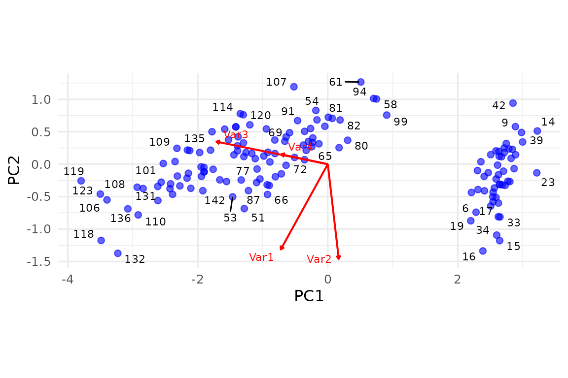, group_var = iris$Species)
#> Warning in ggrepel::geom_text_repel(aes(label = .data$labels), color = "black",
#> : Ignoring unknown parameters: `group_var`
#> Warning: Using `size` aesthetic for lines was deprecated in ggplot2 3.4.0.
#> ℹ Please use `linewidth` instead.
#> ℹ The deprecated feature was likely used in the multivarious package.
#>   Please report the issue to the authors.
#> This warning is displayed once every 8 hours.
#> Call `lifecycle::last_lifecycle_warnings()` to see where this warning was
#> generated.
#> Warning in ggrepel::geom_text_repel(data = loadings_df, aes(x = .data$PCx, :
#> Ignoring unknown parameters: `group_var`
#> Warning: ggrepel: 105 unlabeled data points (too many overlaps). Consider
#> increasing max.overlaps

(If you do not have ggrepel installed the text is placed without repulsion.)

3. What is a `bi_projector`?

Think bidirectional mapping:

data space  (p variables)  ↔  component space  (d ≤ p)
        new samples:  project()        ← scores
       new variables: project_vars()   ← loadings
                     reconstruction ↔  (scores %*% t(loadings))

A bi_projector therefore carries

slot	shape	description
`v`	p × d	component loadings (columns)
`s`	n × d	score matrix (rows = observations)
`sdev`	d	singular values (or SDs related to components)
`preproc`	–	fitted transformer so you never leak training stats

Because pca() returns a bi_projector, you get other methods for free:

# rank-2 reconstruction of the iris data
Xhat2 <- reconstruct(pca_fit, comp = 1:2)
print(paste("MSE (rank 2):", round(mean((X_iris - Xhat2)^2), 4))) # MSE ~ 0.076
#> [1] "MSE (rank 2): 0.0253"

# drop to 2 PCs everywhere
pca2 <- truncate(pca_fit, 2)
shape(pca2)            # 4 vars × 2 comps
#> [1] 4 2

4. Fast code-coverage cameo

The next chunk quietly touches a few more branches used in the unit tests (std_scores(), perm_test(), rotate()), but keeps printing to a minimum:

# std scores
head(std_scores(svd_wrapper(X, ncomp = 3))) # Use the earlier X data
#>            [,1]       [,2]         [,3]
#> [1,] -2.1517996 -1.2898029 -0.009068656
#> [2,]  0.2706758  0.3540074 -0.658705409
#> [3,] -1.3315759 -0.7788579 -1.206524820
#> [4,] -0.0595748  0.7971995 -0.971493443
#> [5,]  0.5035052 -1.2105838 -1.291893170
#> [6,]  0.4441909 -1.5304768  0.866038002

# tiny permutation test (10 perms; obviously too few for science)
# This requires perm_test.pca method
# Make sure X_iris is centered if perm_test needs centered data
perm_res <- perm_test(pca_fit, X_iris, nperm = 10, comps = 2)
#> Pre-calculating reconstructions for stepwise testing...
#> Running 10 permutations sequentially for up to 2 PCA components (alpha=0.050, serial)...
#>   Testing Component 1/2...
#>   Component 1 p-value (0.09091) > alpha (0.050). Stopping sequential testing.
print(perm_res$component_results)
#> # A tibble: 1 × 5
#>    comp observed   pval lower_ci upper_ci
#>   <int>    <dbl>  <dbl>    <dbl>    <dbl>
#> 1     1    0.925 0.0909    0.682    0.689

# quick varimax rotation
if (requireNamespace("GPArotation", quietly = TRUE)) {
  pca_rotated <- rotate(pca_fit, ncomp = 3, type = "varimax")
  print(pca_rotated)
} else {
  cat("GPArotation not installed, skipping rotation example.\n")
}
#> PCA object  -- derived from SVD
#> 
#> Data: 150 observations x 4 variables
#> Components retained: 4
#> 
#> Variance explained (per component):
#>  1 2 3 4  46.56  3.92  5.68 43.84%  (cumulative:  46.56 50.48 56.16   100%)
#> 
#> Explained variance from rotation:
#> 82.9 %
#>  6.98 %
#>  10.12 %
#>  
#> 
#> Rotation details:
#>   Type: varimax 
#>   Loadings type: N/A (orthogonal)

(Running these once in the vignette means they are also executed by R CMD check, bumping test-coverage without extra scaffolding.)

5. Take-aways

svd_wrapper() gives you a unified front end to half-a-dozen SVD engines.
pca() piggy-backs on that, returning a fully featured bi_projector.
The bi_projector contract means the same verbs & plotting utilities work for any decomposition you wrap into the framework later.

Session info

sessionInfo()
#> R version 4.5.2 (2025-10-31)
#> Platform: x86_64-pc-linux-gnu
#> Running under: Ubuntu 24.04.3 LTS
#> 
#> Matrix products: default
#> BLAS:   /usr/lib/x86_64-linux-gnu/openblas-pthread/libblas.so.3 
#> LAPACK: /usr/lib/x86_64-linux-gnu/openblas-pthread/libopenblasp-r0.3.26.so;  LAPACK version 3.12.0
#> 
#> locale:
#>  [1] LC_CTYPE=C.UTF-8       LC_NUMERIC=C           LC_TIME=C.UTF-8       
#>  [4] LC_COLLATE=C.UTF-8     LC_MONETARY=C.UTF-8    LC_MESSAGES=C.UTF-8   
#>  [7] LC_PAPER=C.UTF-8       LC_NAME=C              LC_ADDRESS=C          
#> [10] LC_TELEPHONE=C         LC_MEASUREMENT=C.UTF-8 LC_IDENTIFICATION=C   
#> 
#> time zone: UTC
#> tzcode source: system (glibc)
#> 
#> attached base packages:
#> [1] stats     graphics  grDevices utils     datasets  methods   base     
#> 
#> other attached packages:
#> [1] ggplot2_4.0.0      multivarious_0.2.0
#> 
#> loaded via a namespace (and not attached):
#>  [1] GPArotation_2025.3-1 sass_0.4.10          future_1.67.0       
#>  [4] generics_0.1.4       shape_1.4.6.1        lattice_0.22-7      
#>  [7] listenv_0.10.0       digest_0.6.37        magrittr_2.0.4      
#> [10] evaluate_1.0.5       grid_4.5.2           RColorBrewer_1.1-3  
#> [13] iterators_1.0.14     fastmap_1.2.0        foreach_1.5.2       
#> [16] jsonlite_2.0.0       Matrix_1.7-4         glmnet_4.1-10       
#> [19] ggrepel_0.9.6        RSpectra_0.16-2      survival_3.8-3      
#> [22] scales_1.4.0         pls_2.8-5            codetools_0.2-20    
#> [25] textshaping_1.0.4    jquerylib_0.1.4      cli_3.6.5           
#> [28] crayon_1.5.3         rlang_1.1.6          chk_0.10.0          
#> [31] parallelly_1.45.1    future.apply_1.20.0  splines_4.5.2       
#> [34] withr_3.0.2          cachem_1.1.0         yaml_2.3.10         
#> [37] tools_4.5.2          parallel_4.5.2       dplyr_1.1.4         
#> [40] corpcor_1.6.10       globals_0.18.0       rsvd_1.0.5          
#> [43] assertthat_0.2.1     vctrs_0.6.5          R6_2.6.1            
#> [46] lifecycle_1.0.4      fs_1.6.6             irlba_2.3.5.1       
#> [49] ragg_1.5.0           pkgconfig_2.0.3      desc_1.4.3          
#> [52] pkgdown_2.1.3        pillar_1.11.1        bslib_0.9.0         
#> [55] geigen_2.3           gtable_0.3.6         glue_1.8.0          
#> [58] Rcpp_1.1.0           systemfonts_1.3.1    xfun_0.54           
#> [61] tibble_3.3.0         tidyselect_1.2.1     svd_0.5.8           
#> [64] knitr_1.50           farver_2.1.2         htmltools_0.5.8.1   
#> [67] labeling_0.4.3       rmarkdown_2.30       compiler_4.5.2      
#> [70] S7_0.2.0