Classifying in latent space: k-NN & Random-Forest wrappers
Classifier.Rmd1. Why classify after projection?
Once a dimensionality-reduction model (PCA, PLS, CCA, …) is fitted, every new sample can be projected into the low-dimensional latent space. Running a classifier there – instead of on thousands of noisy raw variables – yields
- fewer parameters & smaller models,
- immunity to collinearity,
- freedom to use partial data (ROI, missing sensors),
- a clean separation between unsupervised decomposition and supervised prediction.
The classifier() S3 family supplied by
multivarious provides that glue: you hand it any projector
(or multiblock_biprojector,
discriminant_projector, …) plus class labels → it returns a
ready predictor object.
2. Iris demo – LDA → discriminant_projector → k-NN
data(iris)
X   <- as.matrix(iris[, 1:4])
grp <- iris$Species

# Hold out a test set up front and fit everything that follows on the
# training rows only, so the held-out accuracy reported later is honest.
set.seed(42)
train_id <- sample(seq_len(nrow(X)), size = 0.7 * nrow(X))
test_id  <- setdiff(seq_len(nrow(X)), train_id)

X_train   <- X[train_id, ]
grp_train <- grp[train_id]

# Fit the centering pre-processor and the LDA on the training data
preproc_fitted <- fit(center(), X_train)
Xp_train       <- transform(preproc_fitted, X_train)
lda_fit        <- MASS::lda(X_train, grouping = grp_train)

# Wrap the LDA result as a discriminant_projector (a bi_projector)
disc_proj <- multivarious::discriminant_projector(
  v       = lda_fit$scaling,              # loadings (p × d)
  s       = Xp_train %*% lda_fit$scaling, # training scores (n_train × d)
  sdev    = lda_fit$svd,                  # singular values
  labels  = grp_train,
  preproc = preproc_fitted                # fitted pre-processor (training means)
)
print(disc_proj)
#> Projector object:
#>   Input dimension: 4
#>   Output dimension: 2
#>   With pre-processing:
#> A finalized pre-processing pipeline:
#>  Step 1: center
#> Label counts:
#>     setosa versicolor  virginica
#>         38         35         32
2.1 Visualise the latent space
scores_df <- as_tibble(scores(disc_proj)[, 1:2],
                       .name_repair = ~ c("LD1","LD2"))
scores_df <- mutate(scores_df, Species = grp_train)

ggplot(scores_df, aes(LD1, LD2, colour = Species)) +
  geom_point(size = 2, alpha = .7) +
  stat_ellipse(level = .9, linewidth = .3) +
  theme_minimal() +
  ggtitle("Iris training set – first two LDA components")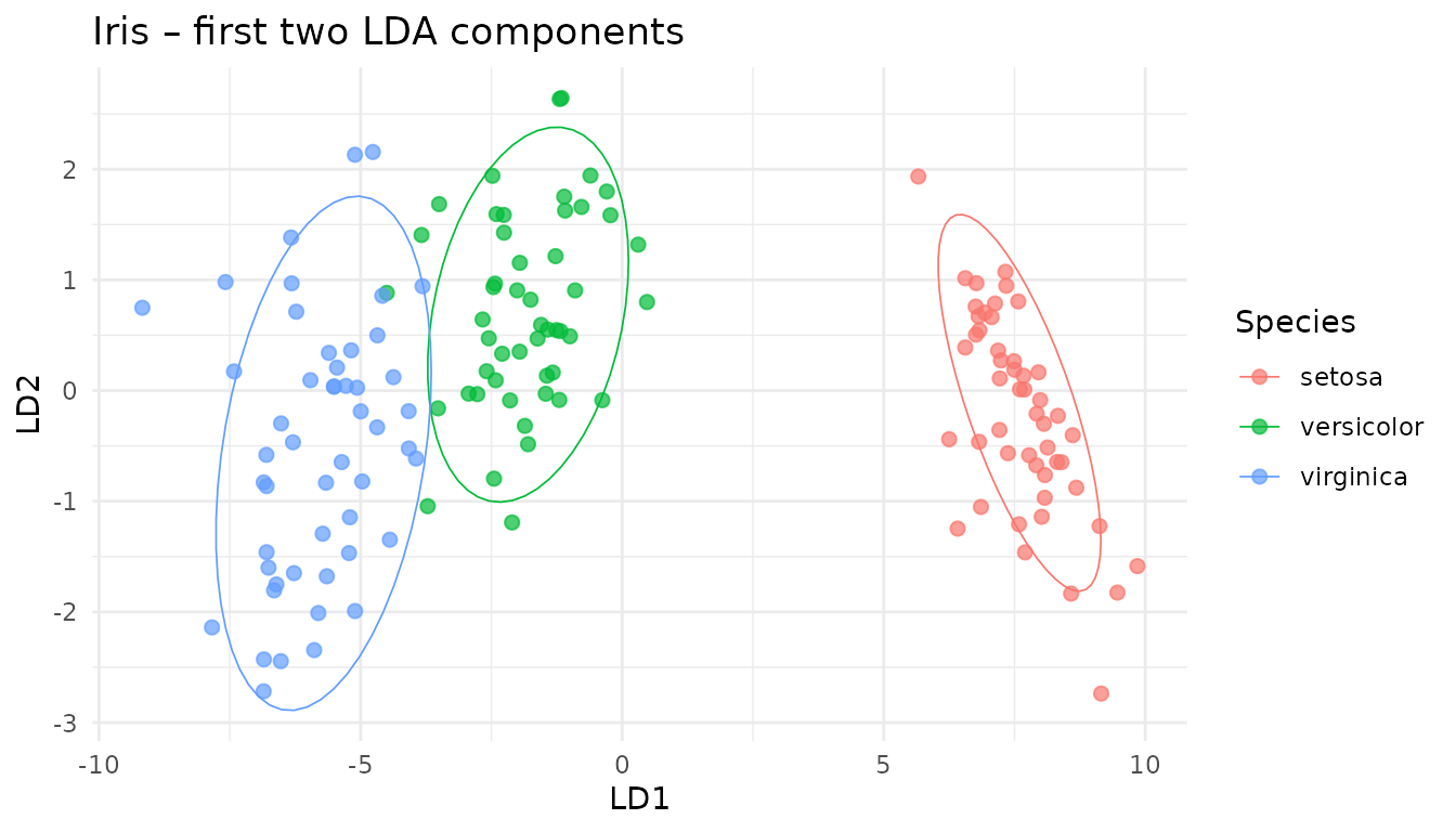
2.2 Build a k-NN classifier on the latent scores
classifier() on a discriminant_projector
uses the projector’s own scores and labels as the reference set. Because
we fitted disc_proj on the training rows, those
are the training scores — no extra arguments are needed.
clf_knn <- multivarious::classifier(disc_proj, knn = 3)
print(clf_knn)
#> k-NN Classifier object:
#>   k-NN Neighbors (k): 3
#>   Number of Training Samples: 105
#>   Number of Classes: 3
#>   Underlying Projector Details:
#>      Projector object:
#>        Input dimension: 4
#>        Output dimension: 2
#>        With pre-processing:
#>      A finalized pre-processing pipeline:
#>       Step 1: center
#>      Label counts:
#>          setosa versicolor  virginica
#>              38         35         32
2.3 Predict and evaluate
pred_knn <- predict(clf_knn, new_data = X[test_id, ],
                    metric = "euclidean", prob_type = "knn_proportion")

head(pred_knn$prob, 3)
#>      setosa versicolor virginica
#> [1,]      1          0         0
#> [2,]      1          0         0
#> [3,]      1          0         0
print(paste("Overall Accuracy:", mean(pred_knn$class == grp[test_id])))
#> [1] "Overall Accuracy: 0.955555555555556"

rk  <- rank_score(pred_knn$prob, grp[test_id])
tk2 <- topk      (pred_knn$prob, grp[test_id], k = 2)

tibble(
  prank_mean = mean(rk$prank),
  top2_acc   = mean(tk2$topk)
)
#> # A tibble: 1 × 2
#>   prank_mean top2_acc
#>        <dbl>    <dbl>
#> 1      0.261        1
2.4 Confusion-matrix on the test set
cm <- table(
  Truth     = grp[test_id],
  Predicted = pred_knn$class
)

# Heat-map
cm_df <- as.data.frame(cm)
ggplot(cm_df, aes(Truth, Predicted, fill = Freq)) +
  geom_tile(colour = "grey80") +
  geom_text(aes(label = Freq), colour = "white", size = 4) +
  scale_fill_gradient(low = "#4575b4", high = "#d73027", name="Count", limits = c(0, 15)) +
  scale_y_discrete(limits = rev(levels(cm_df$Predicted))) +
  theme_minimal(base_size = 12) + coord_equal() +
  ggtitle("k-NN (k = 3) confusion matrix – test set") +
  theme(axis.text.x = element_text(angle = 45, hjust = 1))
# Pretty table as well
knitr::kable(cm, caption = "Confusion matrix (counts)")| setosa | versicolor | virginica | |
|---|---|---|---|
| setosa | 12 | 0 | 0 |
| versicolor | 0 | 14 | 1 |
| virginica | 0 | 1 | 17 |
3. Random-Forest on the same latent space
# rf_classifier() dispatches to the projector method, which takes the
# reference labels and scores explicitly (here, the training scores).
rf_clf <- rf_classifier(
  x      = disc_proj,
  labels = grp_train,
  scores = scores(disc_proj)
)

pred_rf <- predict(rf_clf, new_data = X[test_id, ])
print(paste("RF Accuracy:", mean(pred_rf$class == grp[test_id])))
#> [1] "RF Accuracy: 0.977777777777778"
The RF sees only two input variables (the LDA components) – that keeps trees shallow and speeds-up training.
4. Partial-feature prediction: sepal block only
Assume that in deployment we measure only Sepal variables (cols 1–2). A partial projection keeps the classifier interface unchanged:
sepal_cols <- 1:2

# Create a classifier using reference scores from Sepal columns only
clf_knn_sepal <- multivarious::classifier(
  x       = disc_proj,
  labels  = grp[train_id],
  new_data= X[train_id, sepal_cols],  # Use training data subset
  colind  = sepal_cols,             # Indicate which columns were used
  knn     = 3
)

# Predict using the dedicated sepal classifier
pred_sepal <- predict(
  clf_knn_sepal,                  # Use the sepal-specific classifier
  new_data = X[test_id, sepal_cols]
  # No need for colind here as clf_knn_sepal expects sepal data
)

print(paste("Accuracy (Sepal only):", mean(pred_sepal$class == grp[test_id])))
#> [1] "Accuracy (Sepal only): 0.333333333333333"
Accuracy is lower in this deliberately restricted feature setting, as expected when the strongest Petal measurements are unavailable.
5. Which component block matters most?
feature_importance() can rank variable groups via a
simple “leave-block-out” score drop.
blocks <- list(
  Sepal = 1:2,
  Petal = 3:4
)

fi <- feature_importance(
  clf_knn,
  new_data  = X[test_id, ],
  true_labels = grp[test_id], # Pass the correct test set labels
  blocks    = blocks,
  fun       = rank_score, # Use rank_score as the performance metric
  fun_direction = "lower_is_better",
  approach  = "marginal" # Calculate marginal drop when block is removed
)
print(fi)
#>   block  importance
#> 2   3,4 0.188888889
#> 1   1,2 0.005555556