Partial projection: working with incomplete feature sets
Partial_Projection.Rmd1. Why partial projection?
Assume you trained a dimensionality-reduction model (PCA, PLS, or another projector) on p variables but, at prediction time,
- one sensor is broken,
- a block of variables is too expensive to measure,
- you need a quick first pass while the “heavy” data arrive later.
You still want latent scores in the same component space so downstream summaries, classifiers, or monitoring rules can use the same columns.
This is the role of
partial_project(model, new_data_subset, colind = which.columns)does:
new_data_subset (n × q) ─► project into latent space (n
× k)
with q ≤ p. If the loading vectors are orthonormal this is a simple dot product; otherwise a ridge-regularised least-squares solve is used.
2. Walk-through with a small PCA
set.seed(1)
n  <- 100
p  <- 8
X  <- matrix(rnorm(n * p), n, p)

# Fit a centred 3-component PCA (via SVD)
# Manually center the data and create fitted preprocessor
Xc <- scale(X, center = TRUE, scale = FALSE)
svd_res <- svd(Xc, nu = 0, nv = 3)

# Create a fitted centering preprocessor
preproc_fitted <- fit(center(), X)

pca <- bi_projector(
  v     = svd_res$v,
  s     = Xc %*% svd_res$v,
  sdev  = svd_res$d[1:3], # raw singular values -- matches pca()/svd_wrapper()
  preproc = preproc_fitted
)2.2 Missing two variables ➜ partial projection
Suppose columns 7 and 8 are unavailable for a new batch.
X_miss      <- X[, 1:6]               # keep only first 6 columns
col_subset  <- 1:6                    # their positions in the **original** X

scores_part <- partial_project(pca, X_miss, colind = col_subset)

# How close are the results?
plot_df <- tibble(
  full = scores_full[,1],
  part = scores_part[,1]
)

ggplot(plot_df, aes(full, part)) +
  geom_point() +
  geom_abline(col = "red") +
  coord_equal() +
  labs(title = "Component 1: full vs. partial projection") +
  theme_minimal()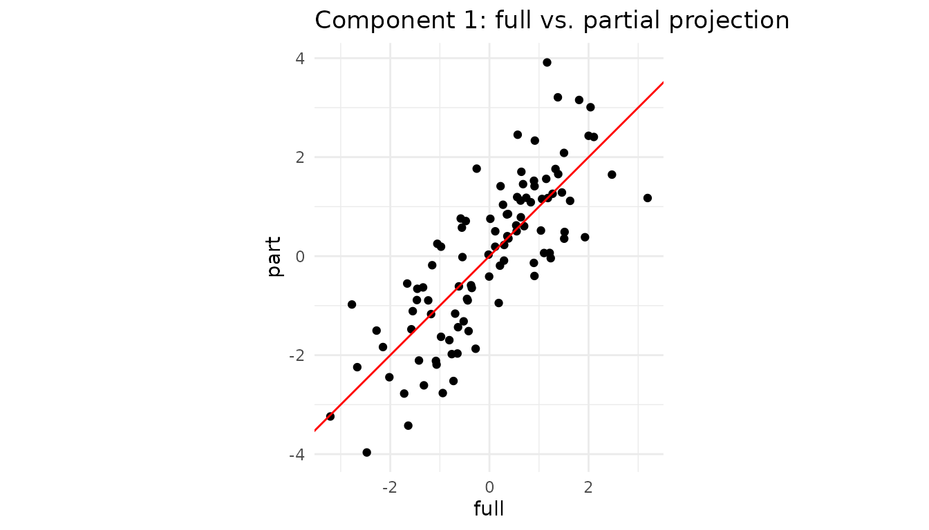
cor(plot_df$full, plot_df$part)
#> [1] 0.8573874
The correlation reports how closely the partial scores agree with the full-data scores for this component.
3. Caching the operation with a partial projector
If you expect many rows with the same subset of features, create a specialised projector once and reuse it:
pca_1to6 <- partial_projector(pca, 1:6)   # keeps a reference + cache

# project 1000 new observations that only have the first 6 vars
new_batch <- matrix(rnorm(1000 * 6), 1000, 6)
scores_fast <- project(pca_1to6, new_batch)
dim(scores_fast)   # 1000 × 3
#> [1] 1000    3
Internally, partial_projector() stores the mapping
v[1:6, ] and a pre-computed inverse, so calls to
project() are as cheap as a matrix multiplication.
4. Block-wise convenience
For multiblock fits (created with
multiblock_projector()), project_block()
provides a convenient wrapper around partial_project():
# Create a multiblock projector from our PCA
# Suppose columns 1-4 are "Block A" (block 1) and columns 5-8 are "Block B" (block 2)
block_indices <- list(1:4, 5:8)

mb <- multiblock_projector(
  v = pca$v,
  preproc = pca$preproc,
  block_indices = block_indices
)

# Now we can project using only Block 2's data (columns 5-8)
X_block2 <- X[, 5:8]
scores_block2 <- project_block(mb, X_block2, block = 2)

# Compare to full projection
head(round(cbind(full = scores_full[,1], block2 = scores_block2[,1]), 2))
#>       full block2
#> [1,] -0.02  -0.36
#> [2,] -2.77  -2.92
#> [3,]  0.57  -0.05
#> [4,] -0.36   0.06
#> [5,]  0.91   1.08
#> [6,]  1.81   1.60
This is equivalent to calling
partial_project(mb, X_block2, colind = 5:8) but reads more
naturally when working with block structures.
5. Not only “missing data”: regions-of-interest & nested designs
Partial projection is handy even when all measurements exist:
- Region of interest (ROI). In neuro-imaging you might have 50,000 voxels but care only about the motor cortex. Projecting just those columns shows how a participant scores within that anatomical region without refitting the whole PCA/PLS.
-
Nested / multi-subject studies. For multi-block PCA
(e.g. “participant × sensor”), you can ask “where would subject i lie if
I looked at block B only?” Supply that block to
project_block(). - Feature probes or “what-if” analysis. Engineers often ask “What is the latent position if I vary only temperature and hold everything else blank?” Pass a matrix that contains the chosen variables and zeros elsewhere.
5.1 Mini-demo: projecting an ROI
Assume columns 1–5 (instead of 50 for brevity) of X form
our ROI.
roi_cols   <- 1:5                 # pretend these are the ROI voxels
X_roi      <- X[, roi_cols]       # same matrix from Section 2

roi_scores <- partial_project(pca, X_roi, colind = roi_cols)

# Compare component 1 from full vs ROI
df_roi <- tibble(
  full = scores_full[,1],
  roi  = roi_scores[,1]
)

ggplot(df_roi, aes(full, roi)) +
  geom_point(alpha = .6) +
  geom_abline(col = "red") +
  coord_equal() +
  labs(title = "Component 1 scores: full data vs ROI") +
  theme_minimal()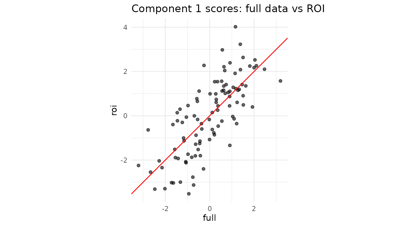
Interpretation: If the two sets of scores align tightly, the ROI variables are driving this component. A strong deviation would reveal that other variables dominate the global pattern.
5.2 Single-subject positioning in a multiblock design
Using the multiblock projector from Section 4, we can see how individual observations score when viewed through just one block:
# Get scores for observation 1 using only Block 1 variables (columns 1-4)
subject1_block1 <- project_block(mb, X[1, 1:4, drop = FALSE], block = 1)

# Get scores for the same observation using only Block 2 variables (columns 5-8)
subject1_block2 <- project_block(mb, X[1, 5:8, drop = FALSE], block = 2)

# Compare: do both blocks tell the same story about this observation?
cat("Subject 1 scores from Block 1:", round(subject1_block1, 2), "\n")
#> Subject 1 scores from Block 1: 0.34 0.43 -0.15
cat("Subject 1 scores from Block 2:", round(subject1_block2, 2), "\n")
#> Subject 1 scores from Block 2: -0.36 0.77 0.64
cat("Subject 1 scores from full data:", round(scores_full[1,], 2), "\n")
#> Subject 1 scores from full data: -0.02 1.2 0.49
This lets you assess whether an observation’s position in the latent space is consistent across blocks, or whether one block tells a different story.
6. Cheat-sheet: why you might call
partial_project()
| Scenario | What you pass | Typical call |
|---|---|---|
| Sensor outage / missing features | matrix with observed cols only | partial_project(mod, X_obs, colind = idx) |
| Region of interest (ROI) | ROI columns of the data | partial_project(mod, X[, ROI], colind = ROI) |
| Block-specific latent scores | full block matrix | project_block(mb, blkData, block = b) |
| “What-if”: vary a single variable set | varied cols + zeros elsewhere |
partial_project() with matching
colind
|
The component space stays identical throughout, so downstream analytics, classifiers, or control charts can continue to use the same score columns without retraining the projector.
Session info
sessionInfo()
#> R version 4.6.1 (2026-06-24)
#> Platform: x86_64-pc-linux-gnu
#> Running under: Ubuntu 24.04.4 LTS
#>
#> Matrix products: default
#> BLAS:   /usr/lib/x86_64-linux-gnu/openblas-pthread/libblas.so.3
#> LAPACK: /usr/lib/x86_64-linux-gnu/openblas-pthread/libopenblasp-r0.3.26.so;  LAPACK version 3.12.0
#>
#> locale:
#>  [1] LC_CTYPE=C.UTF-8       LC_NUMERIC=C           LC_TIME=C.UTF-8
#>  [4] LC_COLLATE=C.UTF-8     LC_MONETARY=C.UTF-8    LC_MESSAGES=C.UTF-8
#>  [7] LC_PAPER=C.UTF-8       LC_NAME=C              LC_ADDRESS=C
#> [10] LC_TELEPHONE=C         LC_MEASUREMENT=C.UTF-8 LC_IDENTIFICATION=C
#>
#> time zone: UTC
#> tzcode source: system (glibc)
#>
#> attached base packages:
#> [1] stats     graphics  grDevices utils     datasets  methods   base
#>
#> other attached packages:
#> [1] ggplot2_4.0.3      dplyr_1.2.1        multivarious_0.4.0
#>
#> loaded via a namespace (and not attached):
#>  [1] Matrix_1.7-5       gtable_0.3.6       jsonlite_2.0.0     compiler_4.6.1
#>  [5] tidyselect_1.2.1   geigen_2.3         jquerylib_0.1.4    systemfonts_1.3.2
#>  [9] scales_1.4.0       textshaping_1.0.5  yaml_2.3.12        fastmap_1.2.0
#> [13] lattice_0.22-9     R6_2.6.1           labeling_0.4.3     generics_0.1.4
#> [17] knitr_1.51         tibble_3.3.1       desc_1.4.3         chk_0.10.0
#> [21] bslib_0.11.0       pillar_1.11.1      RColorBrewer_1.1-3 rlang_1.2.0
#> [25] cachem_1.1.0       xfun_0.59          S7_0.2.2           fs_2.1.0
#> [29] sass_0.4.10        otel_0.2.0         cli_3.6.6          withr_3.0.3
#> [33] pkgdown_2.2.0      magrittr_2.0.5     digest_0.6.39      grid_4.6.1
#> [37] lifecycle_1.0.5    vctrs_0.7.3        evaluate_1.0.5     glue_1.8.1
#> [41] farver_2.1.2       ragg_1.5.2         rmarkdown_2.31     tools_4.6.1
#> [45] pkgconfig_2.0.3    htmltools_0.5.9