Cross-validation for Dimensionality Reduction • multivarious

Why Cross-validate Dimensionality Reduction?

When using PCA or other dimensionality reduction methods, we often face questions like: - How many components should I keep? - How well does my model generalize to new data? - Which preprocessing strategy works best?

Cross-validation provides principled answers by testing how well models trained on one subset of data perform on held-out data.

Quick Example: Finding the Right Number of Components

Let’s use the iris dataset to demonstrate:

# Prepare data
X <- as.matrix(scale(iris[, 1:4]))  # 150 samples × 4 features

# Create 5-fold cross-validation splits
K <- 5
fold_ids <- sample(rep(1:K, length.out = nrow(X)))
folds <- lapply(1:K, function(k) list(
  train = which(fold_ids != k),
  test  = which(fold_ids == k)
))

# Define fitting and measuring functions for PCA cross-validation
fit_pca <- function(train_data, ncomp) {
  pca(train_data, ncomp = ncomp, preproc = center())
}

measure_pca <- function(model, test_data) {
  # Reconstruct test data using the model
  test_scores <- project(model, test_data)
  reconstructed <- reconstruct(model, scores = test_scores)

  # Measure reconstruction error
  measure_reconstruction_error(test_data, reconstructed, metrics = c("rmse"))
}

# Run cross-validation for different numbers of components
results_list <- lapply(1:4, function(ncomp) {
  cv_res <- cv_generic(
    data = X,
    folds = folds,
    .fit_fun = fit_pca,
    .measure_fun = measure_pca,
    fit_args = list(ncomp = ncomp),
    backend = "serial"
  )
  cv_res$ncomp <- ncomp
  cv_res
})
#> Warning in value[[3L]](cond): Measuring failed for fold 1: all(dim(Xtrue) ==
#> dim(Xrec)) is not TRUE
#> Warning in value[[3L]](cond): Measuring failed for fold 2: all(dim(Xtrue) ==
#> dim(Xrec)) is not TRUE
#> Warning in value[[3L]](cond): Measuring failed for fold 3: all(dim(Xtrue) ==
#> dim(Xrec)) is not TRUE
#> Warning in value[[3L]](cond): Measuring failed for fold 4: all(dim(Xtrue) ==
#> dim(Xrec)) is not TRUE
#> Warning in value[[3L]](cond): Measuring failed for fold 5: all(dim(Xtrue) ==
#> dim(Xrec)) is not TRUE
#> Warning in value[[3L]](cond): Measuring failed for fold 1: all(dim(Xtrue) ==
#> dim(Xrec)) is not TRUE
#> Warning in value[[3L]](cond): Measuring failed for fold 2: all(dim(Xtrue) ==
#> dim(Xrec)) is not TRUE
#> Warning in value[[3L]](cond): Measuring failed for fold 3: all(dim(Xtrue) ==
#> dim(Xrec)) is not TRUE
#> Warning in value[[3L]](cond): Measuring failed for fold 4: all(dim(Xtrue) ==
#> dim(Xrec)) is not TRUE
#> Warning in value[[3L]](cond): Measuring failed for fold 5: all(dim(Xtrue) ==
#> dim(Xrec)) is not TRUE
#> Warning in value[[3L]](cond): Measuring failed for fold 1: all(dim(Xtrue) ==
#> dim(Xrec)) is not TRUE
#> Warning in value[[3L]](cond): Measuring failed for fold 2: all(dim(Xtrue) ==
#> dim(Xrec)) is not TRUE
#> Warning in value[[3L]](cond): Measuring failed for fold 3: all(dim(Xtrue) ==
#> dim(Xrec)) is not TRUE
#> Warning in value[[3L]](cond): Measuring failed for fold 4: all(dim(Xtrue) ==
#> dim(Xrec)) is not TRUE
#> Warning in value[[3L]](cond): Measuring failed for fold 5: all(dim(Xtrue) ==
#> dim(Xrec)) is not TRUE
#> Warning in value[[3L]](cond): Measuring failed for fold 1: all(dim(Xtrue) ==
#> dim(Xrec)) is not TRUE
#> Warning in value[[3L]](cond): Measuring failed for fold 2: all(dim(Xtrue) ==
#> dim(Xrec)) is not TRUE
#> Warning in value[[3L]](cond): Measuring failed for fold 3: all(dim(Xtrue) ==
#> dim(Xrec)) is not TRUE
#> Warning in value[[3L]](cond): Measuring failed for fold 4: all(dim(Xtrue) ==
#> dim(Xrec)) is not TRUE
#> Warning in value[[3L]](cond): Measuring failed for fold 5: all(dim(Xtrue) ==
#> dim(Xrec)) is not TRUE

# Combine results
cv_results <- do.call(rbind, lapply(results_list, function(x) {
  data.frame(ncomp = x$ncomp, rmse = mean(x$results$rmse, na.rm = TRUE))
}))
#> Warning: Unknown or uninitialised column: `results`.
#> Warning in mean.default(x$results$rmse, na.rm = TRUE): argument is not numeric
#> or logical: returning NA
#> Warning: Unknown or uninitialised column: `results`.
#> Warning in mean.default(x$results$rmse, na.rm = TRUE): argument is not numeric
#> or logical: returning NA
#> Warning: Unknown or uninitialised column: `results`.
#> Warning in mean.default(x$results$rmse, na.rm = TRUE): argument is not numeric
#> or logical: returning NA
#> Warning: Unknown or uninitialised column: `results`.
#> Warning in mean.default(x$results$rmse, na.rm = TRUE): argument is not numeric
#> or logical: returning NA

# View results
print(cv_results)
#>    ncomp rmse
#> 1      1   NA
#> 2      1   NA
#> 3      1   NA
#> 4      1   NA
#> 5      1   NA
#> 6      2   NA
#> 7      2   NA
#> 8      2   NA
#> 9      2   NA
#> 10     2   NA
#> 11     3   NA
#> 12     3   NA
#> 13     3   NA
#> 14     3   NA
#> 15     3   NA
#> 16     4   NA
#> 17     4   NA
#> 18     4   NA
#> 19     4   NA
#> 20     4   NA

The plot shows that 2 components capture most of the variance, with diminishing returns after that.

Understanding the Output

The cv_generic() function returns a tibble containing:

fold: The fold number
model: The fitted model for each fold (stored as a list column)
metrics: Performance metrics for each fold (stored as a list column of tibbles)

# View the structure of CV results
str(results_list[[1]], max.level = 2)
#> tibble [5 × 4] (S3: tbl_df/tbl/data.frame)
#>  $ fold   : int [1:5] 1 2 3 4 5
#>  $ model  :List of 5
#>  $ metrics:List of 5
#>  $ ncomp  : int [1:5] 1 1 1 1 1

# Extract and combine all metrics across folds
all_fold_metrics <- lapply(results_list, function(res) {
  data.frame(
    ncomp = res$ncomp,
    fold_metrics = dplyr::bind_rows(res$metrics)
  )
})
print(head(all_fold_metrics[[1]]))
#>   ncomp                                    error
#> 1     1 all(dim(Xtrue) == dim(Xrec)) is not TRUE
#> 2     1 all(dim(Xtrue) == dim(Xrec)) is not TRUE
#> 3     1 all(dim(Xtrue) == dim(Xrec)) is not TRUE
#> 4     1 all(dim(Xtrue) == dim(Xrec)) is not TRUE
#> 5     1 all(dim(Xtrue) == dim(Xrec)) is not TRUE

Custom Cross-validation Scenarios

Scenario 1: Comparing Preprocessing Strategies

Use cv_generic() to compare different preprocessing pipelines:

# Define two preprocessing strategies
prep1 <- center()                       # Center only
prep2 <- colscale(center(), type = "z") # Center and scale (z-score)

# Fit function that uses PCA with preprocessing
fit_with_prep <- function(train_data, ncomp, preproc) {
  # PCA will handle preprocessing internally
  pca(train_data, ncomp = ncomp, preproc = preproc)
}

# Measure function that handles preprocessing
measure_with_prep <- function(model, test_data) {
  # Project and reconstruct - PCA handles preprocessing automatically
  scores <- project(model, test_data)
  recon <- reconstruct(model, scores = scores)

  # Calculate metrics
  measure_reconstruction_error(test_data, recon,
                               metrics = c("rmse", "r2"))
}

# Compare both strategies
cv_prep1 <- cv_generic(
  X, folds,
  .fit_fun = fit_with_prep,
  .measure_fun = measure_with_prep,
  fit_args = list(ncomp = 3, preproc = prep1)
)
#> Warning in value[[3L]](cond): Measuring failed for fold 1: all(dim(Xtrue) ==
#> dim(Xrec)) is not TRUE
#> Warning in value[[3L]](cond): Measuring failed for fold 2: all(dim(Xtrue) ==
#> dim(Xrec)) is not TRUE
#> Warning in value[[3L]](cond): Measuring failed for fold 3: all(dim(Xtrue) ==
#> dim(Xrec)) is not TRUE
#> Warning in value[[3L]](cond): Measuring failed for fold 4: all(dim(Xtrue) ==
#> dim(Xrec)) is not TRUE
#> Warning in value[[3L]](cond): Measuring failed for fold 5: all(dim(Xtrue) ==
#> dim(Xrec)) is not TRUE

cv_prep2 <- cv_generic(
  X, folds,
  .fit_fun = fit_with_prep,
  .measure_fun = measure_with_prep,
  fit_args = list(ncomp = 3, preproc = prep2)
)
#> Warning in value[[3L]](cond): Measuring failed for fold 1: all(dim(Xtrue) ==
#> dim(Xrec)) is not TRUE
#> Warning in value[[3L]](cond): Measuring failed for fold 2: all(dim(Xtrue) ==
#> dim(Xrec)) is not TRUE
#> Warning in value[[3L]](cond): Measuring failed for fold 3: all(dim(Xtrue) ==
#> dim(Xrec)) is not TRUE
#> Warning in value[[3L]](cond): Measuring failed for fold 4: all(dim(Xtrue) ==
#> dim(Xrec)) is not TRUE
#> Warning in value[[3L]](cond): Measuring failed for fold 5: all(dim(Xtrue) ==
#> dim(Xrec)) is not TRUE

# Compare results - extract metrics from the tibble
metrics1 <- dplyr::bind_rows(cv_prep1$metrics)
metrics2 <- dplyr::bind_rows(cv_prep2$metrics)

cat("Center only - RMSE:", mean(metrics1$rmse, na.rm = TRUE), "\n")
#> Warning: Unknown or uninitialised column: `rmse`.
#> Warning in mean.default(metrics1$rmse, na.rm = TRUE): argument is not numeric
#> or logical: returning NA
#> Center only - RMSE: NA
cat("Center + Scale - RMSE:", mean(metrics2$rmse, na.rm = TRUE), "\n")
#> Warning: Unknown or uninitialised column: `rmse`.
#> Warning in mean.default(metrics2$rmse, na.rm = TRUE): argument is not numeric
#> or logical: returning NA
#> Center + Scale - RMSE: NA

Scenario 2: Parallel Cross-validation

For larger datasets, run folds in parallel:

# Setup parallel backend
library(future)
plan(multisession, workers = 4)

# Run CV in parallel
cv_parallel <- cv_generic(
  X,
  folds = folds,
  .fit_fun = fit_pca,
  .measure_fun = measure_pca,
  fit_args = list(ncomp = 4),
  backend = "future"  # Use parallel backend
)

# Don't forget to reset
plan(sequential)

Available Metrics

The measure_reconstruction_error() function provides several metrics:

Metric	Description	Range
`mse`	Mean Squared Error	[0, ∞)
`rmse`	Root Mean Squared Error	[0, ∞)
`mae`	Mean Absolute Error	[0, ∞)
`r2`	R-squared (coefficient of determination)	(-∞, 1]

# Define measure function with multiple metrics
measure_pca_multi <- function(model, test_data) {
  test_scores <- project(model, test_data)
  reconstructed <- reconstruct(model, scores = test_scores)
  measure_reconstruction_error(test_data, reconstructed,
                               metrics = c("rmse", "r2", "mae"))
}

# Calculate multiple metrics at once
cv_multi <- cv_generic(
  X,
  folds = folds,
  .fit_fun = fit_pca,
  .measure_fun = measure_pca_multi,
  fit_args = list(ncomp = 4)
)
#> Warning in value[[3L]](cond): Measuring failed for fold 1: all(dim(Xtrue) ==
#> dim(Xrec)) is not TRUE
#> Warning in value[[3L]](cond): Measuring failed for fold 2: all(dim(Xtrue) ==
#> dim(Xrec)) is not TRUE
#> Warning in value[[3L]](cond): Measuring failed for fold 3: all(dim(Xtrue) ==
#> dim(Xrec)) is not TRUE
#> Warning in value[[3L]](cond): Measuring failed for fold 4: all(dim(Xtrue) ==
#> dim(Xrec)) is not TRUE
#> Warning in value[[3L]](cond): Measuring failed for fold 5: all(dim(Xtrue) ==
#> dim(Xrec)) is not TRUE

# View all metrics - extract from list column
all_metrics_multi <- dplyr::bind_rows(cv_multi$metrics)
print(all_metrics_multi)
#> # A tibble: 5 × 1
#>   error                                   
#>   <chr>                                   
#> 1 all(dim(Xtrue) == dim(Xrec)) is not TRUE
#> 2 all(dim(Xtrue) == dim(Xrec)) is not TRUE
#> 3 all(dim(Xtrue) == dim(Xrec)) is not TRUE
#> 4 all(dim(Xtrue) == dim(Xrec)) is not TRUE
#> 5 all(dim(Xtrue) == dim(Xrec)) is not TRUE

# Calculate mean of each metric across folds
cat("\nMean metrics across folds:\n")
#> 
#> Mean metrics across folds:
cat("RMSE:", mean(all_metrics_multi$rmse, na.rm = TRUE), "\n")
#> Warning: Unknown or uninitialised column: `rmse`.
#> Warning in mean.default(all_metrics_multi$rmse, na.rm = TRUE): argument is not
#> numeric or logical: returning NA
#> RMSE: NA
cat("R²:  ", mean(all_metrics_multi$r2, na.rm = TRUE), "\n")
#> Warning: Unknown or uninitialised column: `r2`.
#> Warning in mean.default(all_metrics_multi$r2, na.rm = TRUE): argument is not
#> numeric or logical: returning NA
#> R²:   NA
cat("MAE: ", mean(all_metrics_multi$mae, na.rm = TRUE), "\n")
#> Warning: Unknown or uninitialised column: `mae`.
#> Warning in mean.default(all_metrics_multi$mae, na.rm = TRUE): argument is not
#> numeric or logical: returning NA
#> MAE:  NA

Tips for Effective Cross-validation

1. Preprocessing Inside the Loop

Always fit preprocessing parameters inside the CV loop:

# WRONG: Preprocessing outside CV
X_scaled <- scale(X)  # Uses information from all samples!
cv_wrong <- cv_generic(
  X_scaled, folds,
  .fit_fun = fit_pca,
  .measure_fun = measure_pca,
  fit_args = list(ncomp = 4)
)

# RIGHT: Preprocessing inside CV
# Let PCA handle preprocessing with the preproc parameter
# (See preprocessing comparison example above)

2. Choose Appropriate Fold Sizes

Small datasets (< 100 samples): Use leave-one-out or 10-fold CV
Medium datasets (100-1000): Use 5-10 fold CV
Large datasets (> 1000): Use 3-5 fold CV or hold-out validation

3. Consider Metric Choice

Use RMSE for general reconstruction quality
Use R² to understand proportion of variance explained
Use MAE when outliers are a concern

Advanced: Cross-validating Other Projectors

The CV framework works with any projector type:

# Define fit function for kernel PCA using Nyström approximation
fit_kernel_pca <- function(train_data, ncomp) {
  # Defaults to linear kernel; pass a custom kernel_func if needed
  nystrom_approx(train_data, ncomp = ncomp, nlandmarks = 50)
}

# Define measure function
measure_kernel <- function(model, test_data) {
  test_scores <- project(model, test_data)
  reconstructed <- reconstruct(model, scores = test_scores)
  measure_reconstruction_error(test_data, reconstructed, metrics = c("rmse"))
}

# Cross-validate kernel PCA
cv_kernel <- cv_generic(
  X,
  folds = folds,
  .fit_fun = fit_kernel_pca,
  .measure_fun = measure_kernel,
  fit_args = list(ncomp = 10)
)

# For discriminant analysis with labels (requires passing labels)
fit_lda <- function(train_data, ncomp, labels) {
  discriminant_projector(train_data, labels, ncomp = ncomp)
}

cv_lda <- cv_generic(
  X,
  folds = folds,
  .fit_fun = fit_lda,
  .measure_fun = measure_pca,
  fit_args = list(ncomp = 3, labels = iris$Species)
)

Kernel PCA via Nyström (standard and double)

The nystrom_approx() function provides two variants:

method = "standard": Williams–Seeger single-stage Nyström with the usual scaling
method = "double": Lim–Jin–Zhang two-stage Nyström (efficient when p is large)

With a centered linear kernel and all points as landmarks (m = N), the Nyström eigen-decomposition recovers the exact top eigenpairs of the kernel matrix K = X_c X_c^T. Below is a reproducible snippet that demonstrates this and shows how to project new data.

set.seed(123)
X <- matrix(rnorm(80 * 10), 80, 10)
ncomp <- 5

# Exact setting: linear kernel + centering + m = N
fit_std <- nystrom_approx(
  X, ncomp = ncomp, landmarks = 1:nrow(X), preproc = center(), method = "standard"
)

# Compare kernel eigenvalues: eig(K) vs fit_std$sdev^2
Xc <- transform(fit_std$preproc, X)
K  <- Xc %*% t(Xc)
lam_K <- eigen(K, symmetric = TRUE)$values[1:ncomp]

data.frame(
  component = 1:ncomp,
  nystrom = sort(fit_std$sdev^2, decreasing = TRUE),
  exact_K  = sort(lam_K,          decreasing = TRUE)
)
#>   component   nystrom   exact_K
#> 1         1 117.64481 117.64481
#> 2         2 112.66863 112.66863
#> 3         3 103.44825 103.44825
#> 4         4  83.17891  83.17891
#> 5         5  78.30886  78.30886

# Relationship with PCA: prcomp() returns singular values / sqrt(n - 1)
p <- prcomp(Xc, center = FALSE, scale. = FALSE)
lam_from_pca <- p$sdev[1:ncomp]^2 * (nrow(X) - 1) # equals eig(K)

data.frame(
  component = 1:ncomp,
  from_pca  = sort(lam_from_pca,  decreasing = TRUE),
  exact_K   = sort(lam_K,         decreasing = TRUE)
)
#>   component  from_pca   exact_K
#> 1         1 117.64481 117.64481
#> 2         2 112.66863 112.66863
#> 3         3 103.44825 103.44825
#> 4         4  83.17891  83.17891
#> 5         5  78.30886  78.30886

# Out-of-sample projection for new rows
new_rows <- 1:5
scores_new <- project(fit_std, X[new_rows, , drop = FALSE])
head(scores_new)
#>            [,1]         [,2]        [,3]       [,4]       [,5]
#> [1,] -0.5065700 -0.003782324 -0.89690602 -1.2402365 -0.2466715
#> [2,] -0.3673067  0.489430969 -1.23213982 -1.5330320  0.7247966
#> [3,]  1.9065578 -0.008104080 -0.61654002  1.5191661  1.2188904
#> [4,] -1.5843734 -0.908340577 -0.94045424 -2.8897545 -2.0328659
#> [5,]  0.5690207  0.002415067  0.09988366 -0.0194067  0.5888599

# Double Nyström collapses to standard when l = m = N
fit_dbl <- nystrom_approx(
  X, ncomp = ncomp, landmarks = 1:nrow(X), preproc = center(), method = "double", l = nrow(X)
)
all.equal(sort(fit_std$sdev^2, decreasing = TRUE), sort(fit_dbl$sdev^2, decreasing = TRUE))
#> [1] TRUE

For large feature counts (p >> n), set method = "double" and choose a modest intermediate rank l to reduce the small problem size. Provide a custom kernel_func if you need a non-linear kernel (e.g., RBF).

# Example RBF kernel
gaussian_kernel <- function(A, B, sigma = 1) {
  # ||a-b||^2 = ||a||^2 + ||b||^2 - 2 a·b
  G  <- A %*% t(B)
  a2 <- rowSums(A * A)
  b2 <- rowSums(B * B)
  D2 <- outer(a2, b2, "+") - 2 * G
  exp(-D2 / (2 * sigma^2))
}

fit_rbf <- nystrom_approx(
  X, ncomp = 8, nlandmarks = 40, preproc = center(), method = "double", l = 20,
  kernel_func = gaussian_kernel
)
scores_rbf <- project(fit_rbf, X[1:10, ])

Test coverage for Nyström

This package includes unit tests that validate Nyström correctness:

Standard Nyström recovers the exact kernel eigenpairs when m = N (centered linear kernel)
Double Nyström matches standard when l = m = N
project() reproduces training scores and matches manual formulas for both methods

See tests/testthat/test_nystrom.R in the source for details.

Cross‑validated kernel RMSE: Nyström vs PCA

Below we compare PCA and Nyström (linear kernel) via a kernel‑space RMSE on held‑out folds. For a test block with preprocessed data X_test_c, the true kernel is K_true = X_test_c %*% t(X_test_c). With a rank‑k model, the approximated kernel is K_hat = S %*% t(S), where S are the component scores returned by project().

set.seed(202)

# PCA fit function (reuses earlier fit_pca)
fit_pca <- function(train_data, ncomp) {
  pca(train_data, ncomp = ncomp, preproc = center())
}

# Nyström fit function (standard variant, linear kernel, no RSpectra needed for small data)
fit_nystrom <- function(train_data, ncomp, nlandmarks = 50) {
  nystrom_approx(train_data, ncomp = ncomp, nlandmarks = nlandmarks,
                 preproc = center(), method = "standard", use_RSpectra = FALSE)
}

# Kernel-space RMSE metric for a test fold
measure_kernel_rmse <- function(model, test_data) {
  S <- project(model, test_data)
  K_hat <- S %*% t(S)
  Xc <- reprocess(model, test_data)
  K_true <- Xc %*% t(Xc)
  tibble::tibble(kernel_rmse = sqrt(mean((K_hat - K_true)^2)))
}

# Use a local copy of iris data and local folds for this comparison
X_cv <- as.matrix(scale(iris[, 1:4]))
K <- 5
fold_ids <- sample(rep(1:K, length.out = nrow(X_cv)))
folds_cv <- lapply(1:K, function(k) list(
  train = which(fold_ids != k),
  test  = which(fold_ids == k)
))

# Compare for k = 3 components
k_sel <- 3
cv_pca_kernel <- cv_generic(
  X_cv, folds_cv,
  .fit_fun = fit_pca,
  .measure_fun = measure_kernel_rmse,
  fit_args = list(ncomp = k_sel)
)

cv_nys_kernel <- cv_generic(
  X_cv, folds_cv,
  .fit_fun = fit_nystrom,
  .measure_fun = measure_kernel_rmse,
  fit_args = list(ncomp = k_sel, nlandmarks = 50)
)

metrics_pca <- dplyr::bind_rows(cv_pca_kernel$metrics)
metrics_nys <- dplyr::bind_rows(cv_nys_kernel$metrics)
rmse_pca <- mean(metrics_pca$kernel_rmse, na.rm = TRUE)
rmse_nys <- mean(metrics_nys$kernel_rmse, na.rm = TRUE)

cv_summary <- data.frame(
  method = c("PCA", "Nyström (linear)"),
  kernel_rmse = c(rmse_pca, rmse_nys)
)
print(cv_summary)
#>             method kernel_rmse
#> 1              PCA  0.02153248
#> 2 Nyström (linear)  0.02266859

# Simple bar plot
ggplot(cv_summary, aes(x = method, y = kernel_rmse, fill = method)) +
  geom_col(width = 0.6) +
  guides(fill = "none") +
  labs(title = "Cross‑validated kernel RMSE (k = 3)", y = "Kernel RMSE", x = NULL)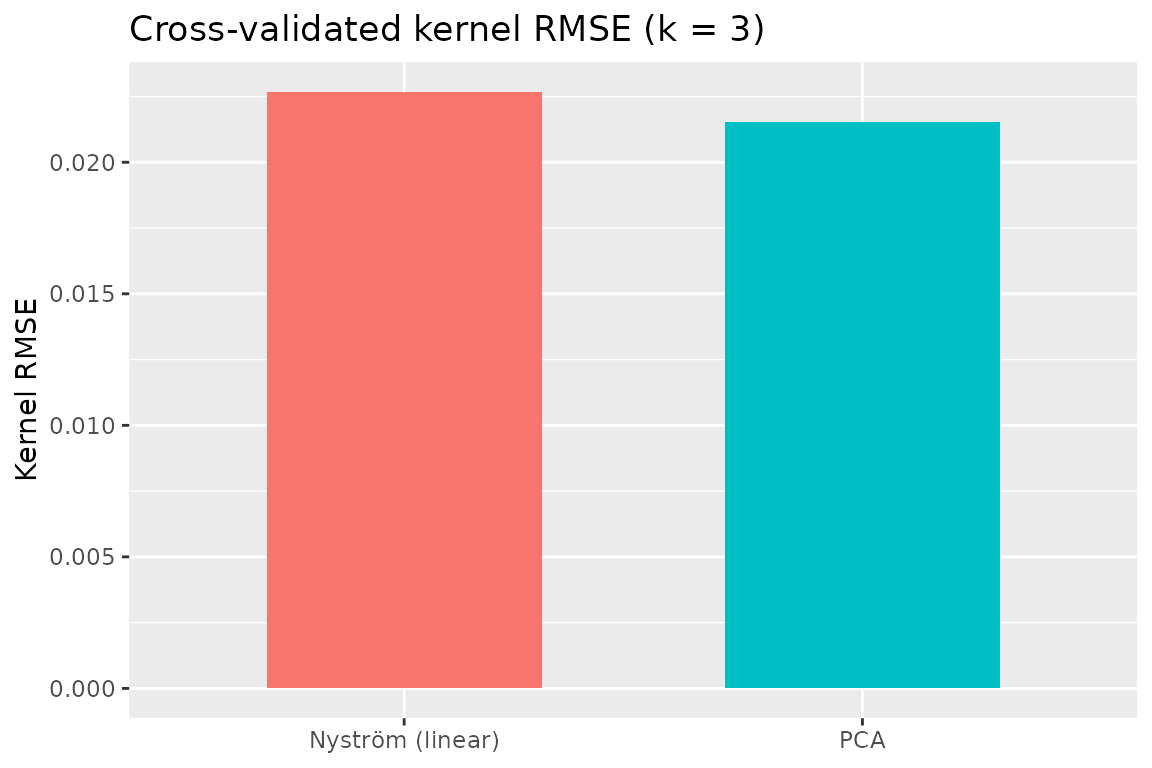

Summary

The multivarious CV framework provides: - Easy cross-validation for any dimensionality reduction method - Flexible metric calculation - Parallel execution support - Tidy output format for easy analysis

Use it to make informed decisions about model complexity and ensure your dimensionality reduction generalizes well to new data.