Contrastive PCA: Finding What's Different Between Groups

What is Contrastive PCA?

Imagine you’re studying two groups: patients with a disease and healthy controls. Both groups show variation in their measurements, but you’re specifically interested in what makes the patients different. Standard PCA would find the largest sources of variation across all samples, which might be dominated by age, sex, or other factors common to both groups.

Contrastive PCA (cPCA++) finds patterns that are enriched in one group (foreground) compared to another (background).

A Worked Example

The simulation below separates variation that is common to both groups from variation that is added only to the foreground group.

set.seed(123)
n_samples <- 100
n_features <- 50

# Create background data (e.g., healthy controls)
# Main variation is in features 1-10
background <- matrix(rnorm(n_samples * n_features), n_samples, n_features)
background[, 1:10] <- background[, 1:10] * 3  # Strong common variation

# Create foreground data (e.g., patients)
# Has the same common variation PLUS disease-specific signal in features 20-25
foreground <- background[1:60, ]  # Start with same structure
foreground[, 20:25] <- foreground[, 20:25] + matrix(rnorm(60 * 6, sd = 2), 60, 6)

# Standard PCA on combined data
all_data <- rbind(background, foreground)
regular_pca <- pca(all_data, ncomp = 2)

# Contrastive PCA
cpca_result <- cPCAplus(X_f = foreground, X_b = background, ncomp = 2)
#> Using feature-space strategy...

# Compare what each method finds
loadings_df <- rbind(
  data.frame(
    feature = factor(1:30),
    value   = abs(regular_pca$v[1:30, 1]),
    method  = "Standard PCA"
  ),
  data.frame(
    feature = factor(1:30),
    value   = abs(cpca_result$v[1:30, 1]),
    method  = "Contrastive PCA"
  )
)

ggplot(loadings_df, aes(x = feature, y = value)) +
  geom_col(fill = "#1f78b4") +
  facet_wrap(~method, nrow = 1) +
  theme_minimal(base_size = 12) +
  theme(axis.text.x = element_text(angle = 45, hjust = 1)) +
  labs(
    x = "Feature",
    y = "|Loading|",
    title = "Top loading coefficients for PC1"
  )

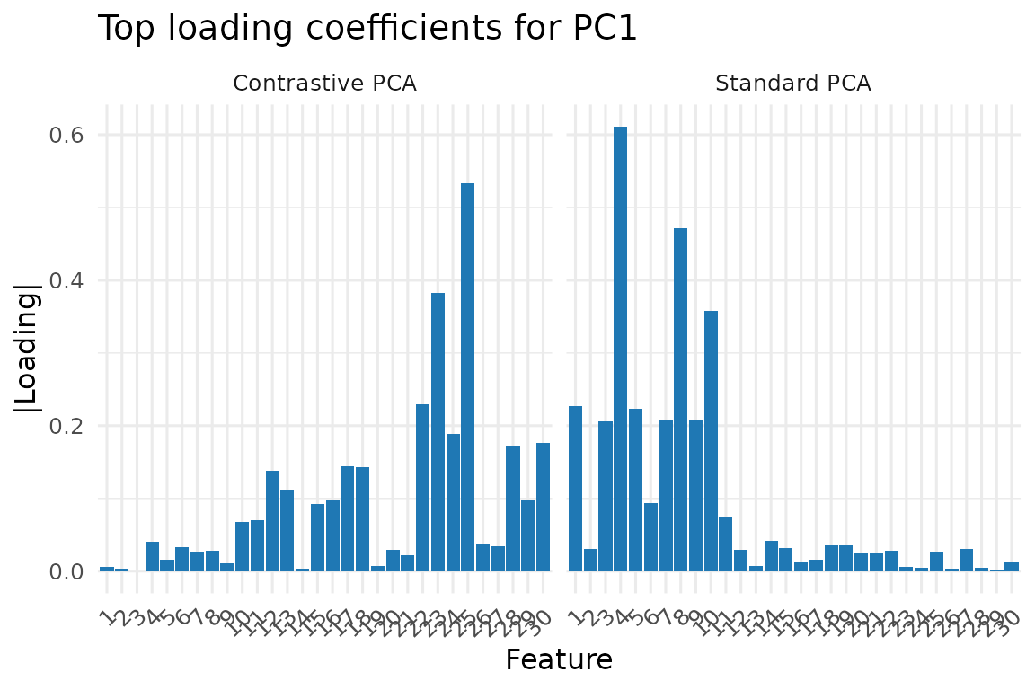
In this draw, standard PCA concentrates on the shared high-variance features near 1-10. The contrastive solution shifts its largest loadings toward the foreground-specific block around 20-25, although individual top-ranked features can vary because the signal is noisy.

Using cPCAplus()

The standard call supplies foreground data, background data, and the number of contrastive components to estimate:

# Basic usage
cpca_fit <- cPCAplus(
  X_f = foreground,  # Your group of interest (foreground)
  X_b = background,  # Your reference group (background)
  ncomp = 5          # Number of components to extract
)
#> Using feature-space strategy...

# The result is a bi_projector object with familiar methods
print(cpca_fit)
#> A bi_projector object with the following properties:
#> 
#> Dimensions of the weights (v) matrix:
#>   Rows:  50  Columns:  5 
#> 
#> Dimensions of the scores (s) matrix:
#>   Rows:  60  Columns:  5 
#> 
#> Length of the standard deviations (sdev) vector:
#>   Length:  5 
#> 
#> Preprocessing information:
#> A finalized pre-processing pipeline:
#>  Step 1: center

# Project new data
new_samples <- matrix(rnorm(10 * n_features), 10, n_features)
new_scores <- project(cpca_fit, new_samples)

# Reconstruct using top components
reconstructed <- reconstruct(cpca_fit, comp = 1:2)

Understanding the Output

cPCAplus() returns a bi_projector object containing:

v: Loadings (feature weights) for each component
s: Scores (sample projections) for the foreground data
sdev: Standard deviations explaining the “contrastive variance”
values: The eigenvalue ratios (foreground variance / background variance)

# Which features contribute most to the first contrastive component?
top_features <- order(abs(cpca_fit$v[, 1]), decreasing = TRUE)[1:10]
print(paste("Top contributing features:", paste(top_features, collapse = ", ")))
#> [1] "Top contributing features: 25, 23, 42, 32, 22, 24, 50, 30, 28, 33"

# How much more variable is each component in foreground vs background?
print(paste("Variance ratios:", paste(round(cpca_fit$values[1:3], 2), collapse = ", ")))
#> [1] "Variance ratios: 16.74, 13.31, 10.31"

Common Applications

Use contrastive PCA when the foreground and background matrices have the same columns and the scientific question is about variance enriched in the foreground. Common examples include disease versus control samples, biological replicates versus technical replicates, or post-treatment versus pre-treatment measurements. In each case, put the group of interest in X_f and the reference or nuisance group in X_b.

Advanced Options

Handling High-Dimensional Data

When you have more features than samples (p >> n), use the efficient sample-space strategy:

# Create high-dimensional example
n_f <- 50; n_b <- 80; p <- 1000
X_background_hd <- matrix(rnorm(n_b * p), n_b, p)
X_foreground_hd <- X_background_hd[1:n_f, ] + 
                   matrix(c(rnorm(n_f * 20, sd = 2), rep(0, n_f * (p-20))), n_f, p)

# Use sample-space strategy for efficiency
cpca_hd <- cPCAplus(X_f = X_foreground_hd, X_b = X_background_hd,
                    ncomp = 5, strategy = "sample")
#> Using sample-space strategy...
#> Warning in irlba::irlba(X_b_centered, nv = r_target, nu = 0): You're computing
#> too large a percentage of total singular values, use a standard svd instead.

Regularization for Unstable Background

If your background covariance is nearly singular, add regularization:

# Small background sample size can lead to instability
small_background <- matrix(rnorm(20 * 100), 20, 100)
small_foreground <- matrix(rnorm(30 * 100), 30, 100)

# Add regularization
cpca_regularized <- cPCAplus(
  X_f = small_foreground,
  X_b = small_background,
  ncomp = 5,
  lambda = 0.1  # Regularization parameter for background covariance
)
#> Using feature-space strategy...

When to Use Contrastive PCA

✓ Use contrastive PCA when: - You have two groups and want to find patterns specific to one - Background variation obscures your signal of interest - You want to remove technical/batch effects captured by control samples

✗ Don’t use contrastive PCA when: - You only have one group (use standard PCA) - Groups differ mainly in mean levels (use t-tests or LDA) - The interesting variation is non-linear (consider kernel methods)

Technical Details

Click for mathematical details

Contrastive PCA++ solves the generalized eigenvalue problem:

$\mathbf{R}_f \mathbf{v} = \lambda \mathbf{R}_b \mathbf{v}$

where: - $\mathbf{R}_f$ is the foreground covariance matrix - $\mathbf{R}_b$ is the background covariance matrix - $\lambda$ represents the variance ratio (foreground/background) - $\mathbf{v}$ are the contrastive directions

This finds directions that maximize the ratio of foreground to background variance, effectively highlighting patterns enriched in the foreground group.

The geneig() function provides the underlying solver with multiple algorithm options: - "geigen": General purpose, handles non-symmetric matrices - "robust": Fast for well-conditioned problems - "rspectra": Efficient for very large sparse matrices

References

Abid, A., Zhang, M. J., Bagaria, V. K., & Zou, J. (2018). Exploring patterns enriched in a dataset with contrastive principal component analysis. Nature Communications, 9(1), 2134.
Salloum, R., & Kuo, C. C. J. (2022). cPCA++: An efficient method for contrastive feature learning. Pattern Recognition, 124, 108378.
Wu, M., Sun, Q., & Yang, Y. (2025). PCA++: How Uniformity Induces Robustness to Background Noise in Contrastive Learning. arXiv preprint arXiv:2511.12278.
Woller, J. P., Menrath, D., & Gharabaghi, A. (2025). Generalized contrastive PCA is equivalent to generalized eigendecomposition. PLOS Computational Biology, 21(10), e1013555.