Neuroimaging Atlases and Parcellations • neuroatlas

neuroatlas provides a unified interface for working with neuroimaging atlases and parcellations in R. Whether you’re conducting ROI-based analyses, visualizing brain data, or integrating different parcellation schemes, neuroatlas streamlines these tasks with consistent, user-friendly functions.

Features

Many built-in atlases: Schaefer (100-1000 parcels), Brainnetome (246 regions), Glasser (360 regions), HCPex (426 regions), Harvard-Oxford, Julich-Brain, FreeSurfer ASEG, harmonized TemplateFlow/AtlasPack subcortical atlases, Olsen MTL, and probabilistic visual-cortex atlases (Wang 2015, visfAtlas, cytoarchitectonic V1-V5)
Surface & volume: Work with both volumetric and surface-based parcellations through one consistent interface
Atlas discovery: Enumerate built-ins with list_atlases() and load any of them by name with get_atlas()
ROI analysis: Extract and summarise regions with get_roi(), map_atlas(), reduce_atlas(), and batch_reduce()
Atlas operations: Combine and reshape parcellations with merge_atlases(), filter_atlas(), dilate_atlas(), atlas_overlap(), and resampling across spaces/resolutions
Template transforms: Resolve verified image-space transforms, resample labels or continuous/probability volumes, and keep artifact and interpolation receipts
Spatial queries: Look up parcels by world, voxel, or MNI coordinate with query_point(), query_coord(), and query_vox()
Network & graph tools: atlas_connectivity(), atlas_graph() / as_igraph(), atlas_hierarchy(), and spin_test() spatial null models
TemplateFlow integration: Access standardized templates through the pure-R templateflow backend
Visualization: Publication-quality surface figures with plot_brain() / plot_brain_grid(), sulcal shading from topology-checked white-surface curvature (surface_anatomy()), perceptually-optimised ROI palettes, the ggseg ecosystem, and an interactive cluster_explorer() Shiny app
Metadata: Atlases and loaded templates carry identity, spatial geometry, citations, source artifacts, and processing history (atlas_metadata(), template_metadata()).

Installation

You can install the development version from GitHub:

# install.packages("pak")
pak::pak("bbuchsbaum/neuroatlas")

TemplateFlow Setup

TemplateFlow access uses the imported pure-R templateflow package. No Python or reticulate setup is required:

neuroatlas::tflow_spaces(pattern = "^MNI")
neuroatlas::show_templateflow_cache_path()

Quick Start

library(neuroatlas)

# Get a Schaefer atlas (200 parcels, 7 networks)
schaefer <- get_schaefer_atlas(parcels = 200, networks = 7)
print(schaefer)

# Extract a specific ROI by label (e.g. the first visual parcel)
roi <- get_roi(schaefer, "Vis_1")

# Get Glasser atlas
glasser <- get_glasser_atlas()

# Access templates via TemplateFlow
mni_brain <- get_template("MNI152NLin2009cAsym", variant = "brain")

Discovering and loading atlases

# See every built-in atlas
list_atlases()

# Load any of them by id (with loader-specific arguments)
schaefer <- get_atlas("schaefer2018", parcels = "100", networks = "7")

HCPex: cortex and subcortex

HCPex adds 66 subcortical regions to the 360 cortical regions of HCP-MMP1.0. Load the upstream v1.1 volume at 1 or 2 mm:

hcp <- get_atlas("hcpex", resolution = 2)
get_roi(hcp, label = "V1_L")
subcortex <- filter_atlas(hcp, division == "subcortical")
roi_metadata(subcortex)  # Abbreviations, full names, hemisphere, and colors
atlas_citations(hcp)

The source declares MNI152NLin2009cAsym template space. HCPex uses its own region ordering; reorder matrices from original HCP-MMP1.0 order before mapping them to this atlas. Downloads are cached and checked against pinned checksums. The upstream atlas data are licensed under GPL-3.0.

Identify and cite a resource

aseg <- get_aseg_atlas()
atlas_metadata(aseg)       # Identity, current geometry, source, and modifications
atlas_citations(aseg)      # R bibliography entries, ready for toBibtex()
atlas_artifacts(aseg)      # Original files, license information, and checksums
atlas_history(aseg)        # Recorded operations and their parameters

Metadata stay attached when objects are saved. Source-file geometry and current object geometry are recorded separately, and unknown provenance is explicit. See Identify, cite, and trace an atlas.

Move an atlas to another template

transform_atlas() preserves region IDs and samples labels on the target grid. Check space_transform_manifest() for available routes. The transform engine is an optional dependency; install the pinned revision used for qualification:

pak::pak(c("hdf5r",
  "bbuchsbaum/neurotransform@933edddda462593941e167726e8aaa7168ff103a"))

schaefer <- get_schaefer_atlas(parcels = 200, networks = 7, resolution = 2)
aligned <- transform_atlas(
  schaefer, "MNI152NLin2009cAsym", resolution = 2, provider = "neuroatlas"
)
attr(aligned, "neuroatlas_transform")$lost_label_ids

Both MNI152NLin6Asym / MNI152NLin2009cAsym directions are available from the qualified artifact release. Qualification covers 1 mm and 2 mm target grids. Each transform is about 86 MiB, downloaded once and checked against its pinned SHA-256 digest. Subsequent calls can use offline = TRUE with a cached transform and an explicit target grid. For scalar or probability volumes, use get_template_transform() and apply_template_transform() with explicit sampling semantics. Probability channels are interpolated independently without renormalization. Template-derived artifacts have separate distribution conditions.

An image-space transform does not establish correspondence between different parcellations. Use atlas_overlap() after alignment to compare their regions. See Verified template transforms.

Map exact cortical domains

The pinned fsaverage 164k and fsLR 32k domains support directed native surface resampling in both hemispheres. Exact geometry identifies vertex ordering, registration, cortical masks and method; a broad name such as "fsaverage" does not admit a route. Install the pinned engine above and optional gifti.

source <- get_surface_geometry("fsaverage", "164k", "L")
target <- get_surface_geometry("fsLR", "32k", "L")
operator <- get_template_transform(source, target)
metric <- surface_data(rep(0.25, source$domain$n_vertices), source$domain)
mapped <- apply_template_transform(metric, operator)
mapped$coverage$available

# Population cortical projection preserves atlas region IDs and names.
atlas <- get_harvard_oxford_atlas("cortical", threshold = 25, resolution = "02")
cortex <- transform_atlas(atlas, target)
cortex$label_table

Population projection supports exact MNI152NLin6Asym and MNI152NLin2009cAsym sources. Numerical qualification covers their locked 1 mm and 2 mm grids. Labels use nearest voxel sampling and categorical surface votes; continuous and probability maps use trilinear sampling. Unsupported cortical values remain NA; supported zero is valid. Outputs record coverage, lost labels, input hashes and directed provenance. Verified inputs and operators can be replayed with offline = TRUE.

ribbon_projection() separately declares ordered white/pial coordinates aligned with a source volume. The caller supplies that alignment; this function does not fit registration. Population projection and numerical agreement do not establish subject registration, anatomical accuracy, area conservation or a lossless inverse. The native surface method has separate qualification from Workbench’s area-aware resampling. Input assets retain their upstream licenses.

Palette demos

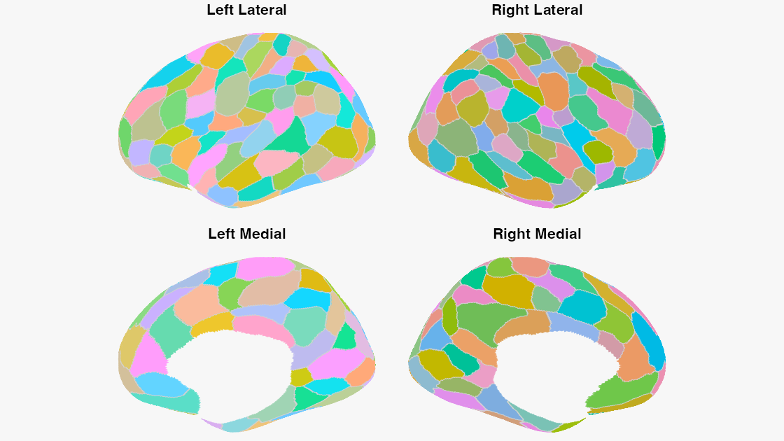
neuroatlas includes perceptually-optimised palettes for atlas ROIs. For instance, you can generate a slice-aware palette for the Schaefer 200×7 atlas and feed it directly into plot_brain():

library(neuroatlas)

schaefer <- get_schaefer_atlas(parcels = 200, networks = 7)

colors <- atlas_roi_colors(
  schaefer,
  method = "maximin_view",
  seed = 1
)

schaefer_surface <- schaefer_surf(parcels = 200, networks = 7)

plot_brain(
  schaefer_surface,
  colors = colors,
  interactive = FALSE,
  style = "ggseg_like"
)

Schaefer-200 (7-network) parcellation on the fsaverage6 surface with a perceptually-optimised maximin colour palette; lateral and medial views of both hemispheres.

Anatomical shading

CPU renders of inflated surfaces shade sulci and gyri from mean curvature of the matching white mesh. Shading is applied only when the two meshes share a topology. Use surface_anatomy() to inspect the metric and its provenance, or to supply your own per-vertex sulcal depth. Tune the underlay with the anatomy_* arguments of plot_brain():

anat <- surface_anatomy(schaefer_surface, hemi = "lh")
anat$provenance$source  # "computed_mean_curvature"

plot_brain(
  schaefer_surface,
  interactive = FALSE,
  anatomy_range = c(0.65, 0.92)
)

Available Atlases

Atlas	Function	Description
Schaefer	`get_schaefer_atlas()`	Cortical parcellations (100-1000 regions, 7 or 17 networks); surface via `get_schaefer_surfatlas()`
Brainnetome	`get_brainnetome_atlas()`	246-region connectional atlas with Yeo network and cytoarchitectonic metadata
Glasser	`get_glasser_atlas()`	360-region multi-modal cortical parcellation (surface via `glasser_surf()`)
HCPex	`get_hcpex_atlas()`	360 cortical and 66 subcortical regions, native 1/2 mm volumes in MNI152NLin2009cAsym
Harvard-Oxford	`get_harvard_oxford_atlas()`	Cortical/subcortical structural atlases via TemplateFlow or FSL
Julich-Brain	`get_julich_brain_atlas()`	FSL Julich-Brain cytoarchitectonic atlas
ASEG	`get_aseg_atlas()`	FreeSurfer subcortical segmentation
Subcortical	`get_subcortical_atlas()`	Harmonized thalamus, cerebellum, and subcortex atlases (AtlasPack/TemplateFlow)
Olsen MTL	`get_olsen_mtl()`	Medial temporal lobe atlas with hippocampal subfields
Wang (2015)	`get_wang_atlas()`	Probabilistic visual topography on `fsaverage` (25 areas/hemi); probability volumes via `get_wang_prob_atlas()`
visfAtlas	`get_visfatlas()`	Probabilistic functional atlas of occipito-temporal visual cortex (33 regions)
Visual V1-V5	`get_visual_atlas()`	Cytoarchitectonic early visual areas extracted from Julich-Brain

Documentation

Getting Started - Introduction and basic usage
Atlas Visualization with Optimal Colours - Perceptually-optimised ROI palettes
Surface Panel Figures - Static panel composition with plot_brain() and plot_brain_grid()
Surface Templates - Geometry vs. data on surface meshes
Surface Parcellations - Surface-based atlas operations
Verified Template Transforms - Align volumes and atlases on explicit grids
Working with TemplateFlow - Template access and management
Function Reference - Complete API documentation

neuroim2 - Core neuroimaging data structures
neurosurf - Surface-based operations
ggseg - Brain visualization

License

Albers theme

This package uses the albersdown theme. Existing vignette theme hooks are replaced so albers.css and local albers.js render consistently on CRAN and GitHub Pages. The palette family is provided via params$family (default ‘red’). The pkgdown site uses template: { package: albersdown }.

neuroatlas