Efficient Clustered fMRI Storage with H5ParcellatedMultiScan

library(fmristore)
#> 
#> Attaching package: 'fmristore'
#> The following object is masked from 'package:stats':
#> 
#>     offset
library(neuroim2)
#> Loading required package: Matrix
#> 
#> Attaching package: 'neuroim2'
#> The following object is masked from 'package:base':
#> 
#>     scale

What is H5ParcellatedMultiScan?

The H5ParcellatedMultiScan class stores multiple fMRI runs where brain voxels have been organized into spatial clusters (e.g., brain parcels, ROIs, or atlas regions). This approach is perfect for:

Multi-run studies with consistent spatial organization across runs
ROI-based analyses where you care about specific brain regions
Memory efficiency when working with large datasets
Fast access to time series from brain regions of interest

Think of it as organizing your fMRI data like a filing cabinet: instead of having one giant drawer with all voxels mixed together, you have separate folders for each brain region, making it much faster to find what you need.

Simple Example: From Data to Storage

Let’s start with the simplest possible workflow - creating some dummy data and saving it.

Step 1: Create Brain Data

# Create a tiny "brain" for this example (10×10×5 voxels)
brain_dims <- c(10, 10, 5)
brain_space <- NeuroSpace(brain_dims, spacing = c(2, 2, 2))

# Define which voxels contain "brain tissue" (a simple box in the center)
mask_data <- array(FALSE, brain_dims)
mask_data[4:7, 4:7, 2:4] <- TRUE # Small 4×4×3 "brain"
mask <- LogicalNeuroVol(mask_data, brain_space)

cat("Our tiny brain has", sum(mask), "voxels\n")
#> Our tiny brain has 48 voxels

Step 2: Create Brain Regions (Clusters)

# Divide our brain into 3 regions
n_voxels <- sum(mask)
cluster_assignments <- rep(1:3, length.out = n_voxels)

# Create the clustered volume
clusters <- ClusteredNeuroVol(mask, cluster_assignments)

# See how many voxels are in each region
print(table(clusters@clusters))
#> 
#>  1  2  3 
#> 16 16 16

Step 3: Create Some fMRI Data

# Create a 4D fMRI dataset (our 3D brain + time dimension)
n_timepoints <- 50
fmri_dims <- c(brain_dims, n_timepoints)

# Generate realistic-looking fMRI data (random but with some structure)
fmri_data <- array(rnorm(prod(fmri_dims)), dim = fmri_dims)

# Make the signal different in each cluster (so we can tell them apart)
for (i in 1:3) {
  cluster_voxels <- which(clusters@clusters == i)
  mask_indices <- which(mask, arr.ind = TRUE)

  for (v in cluster_voxels) {
    x <- mask_indices[v, 1]
    y <- mask_indices[v, 2]
    z <- mask_indices[v, 3]
    # Add a small bias to each cluster
    fmri_data[x, y, z, ] <- fmri_data[x, y, z, ] + i * 0.5
  }
}

# Convert to NeuroVec (the fmristore format for 4D data)
nvec <- NeuroVec(fmri_data, NeuroSpace(fmri_dims))
cat("Created fMRI data with dimensions:", paste(dim(nvec), collapse = " × "), "\n")
#> Created fMRI data with dimensions: 10 × 10 × 5 × 50

Step 4: Save Using the New Simple Interface

# Save to HDF5 using the new write_dataset() function
output_file <- tempfile(fileext = ".h5")

# This is the new simplified way to save clustered data
# Note: mask is extracted from the clusters object automatically
write_dataset(nvec, file = output_file, clusters = clusters)
#> Creating HDF5 file: /tmp/Rtmpk1VJ8c/file22da72a8f305.h5
#> Writing global structures (mask, clusters, header)...
#> Writing scan data...
#>   Writing scan: scan_001 (type: full)
#>     Scan 'scan_001': nTime not in metadata, attempting to infer from sdata list.
#>     Scan 'scan_001': Inferred nTime 50 from sdata item 'cluster_1'.

cat("Data saved to:", basename(output_file), "\n")
#> Data saved to: file22da72a8f305.h5
cat("File size:", round(file.size(output_file) / 1024, 1), "KB\n")
#> File size: 33.7 KB

Step 5: Load Using the New Simple Interface

# Use the new read_dataset() function with automatic type detection
experiment <- read_dataset(output_file)
#> Detected type 'H5ParcellatedMultiScan' in file: /tmp/Rtmpk1VJ8c/file22da72a8f305.h5
#> Clusters argument is NULL, attempting to read from HDF5 file (/cluster_map).

# Show what we got back
experiment
#> 
#> H5ParcellatedMultiScan
#>   # runs        : 1 
#>   # clusters    : 0 
#>   mask dims     : 10x10x5 
#>   HDF5 file     : /tmp/Rtmpk1VJ8c/file22da72a8f305.h5

# The function automatically detected this is a parcellated experiment
cat("Detected type:", class(experiment), "\n")
#> Detected type: H5ParcellatedMultiScan
cat("Number of runs:", n_scans(experiment), "\n")
#> Number of runs: 1
cat("Available scan names:", paste(scan_names(experiment), collapse = ", "), "\n")
#> Available scan names: scan_001

Step 6: Extract and Visualize Data

# Get the first (and only) run
my_run <- experiment@runs[[1]]

# Extract time series from the first few voxels
voxel_data <- series(my_run, i = 1:6)
cat("Time series dimensions:", paste(dim(voxel_data), collapse = " × "), "\n")
#> Time series dimensions: 50 × 6
cat("(rows = time points, columns = voxels)\n\n")
#> (rows = time points, columns = voxels)

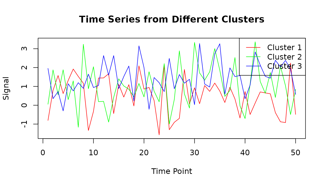
# Plot time series from different clusters to see they're different
matplot(voxel_data[, 1:3],
  type = "l",
  main = "Time Series from Different Clusters",
  xlab = "Time Point", ylab = "Signal",
  col = c("red", "green", "blue"), lty = 1
)
legend("topright",
  legend = paste("Cluster", 1:3),
  col = c("red", "green", "blue"), lty = 1
)

Advanced Example: Multiple Runs with Summary Data

Now let’s see a more realistic example with multiple runs and both detailed and summarized data.

Create Multiple Runs

# Create 3 different fMRI runs with different characteristics
run_names <- c("rest", "task1", "task2")
runs_data <- list()

for (i in 1:3) {
  # Each run has different length and characteristics
  n_time <- 40 + i * 10 # 50, 60, 70 timepoints
  run_dims <- c(brain_dims, n_time)

  # Generate data with run-specific patterns
  run_data <- array(rnorm(prod(run_dims)), dim = run_dims)

  # Add different activation patterns for each run
  if (i == 2) {
    # Task1: stronger activation in cluster 2
    cluster_2_voxels <- which(clusters@clusters == 2)
    mask_indices <- which(mask, arr.ind = TRUE)
    for (v in cluster_2_voxels) {
      x <- mask_indices[v, 1]
      y <- mask_indices[v, 2]
      z <- mask_indices[v, 3]
      run_data[x, y, z, ] <- run_data[x, y, z, ] + sin(seq(0, 2 * pi, length.out = n_time))
    }
  } else if (i == 3) {
    # Task2: stronger activation in cluster 3
    cluster_3_voxels <- which(clusters@clusters == 3)
    mask_indices <- which(mask, arr.ind = TRUE)
    for (v in cluster_3_voxels) {
      x <- mask_indices[v, 1]
      y <- mask_indices[v, 2]
      z <- mask_indices[v, 3]
      run_data[x, y, z, ] <- run_data[x, y, z, ] + cos(seq(0, 2 * pi, length.out = n_time))
    }
  }

  runs_data[[i]] <- NeuroVec(run_data, NeuroSpace(run_dims))
}

cat(
  "Created", length(runs_data), "runs with",
  paste(sapply(runs_data, function(x) dim(x)[4]), collapse = ", "), "timepoints\n"
)
#> Created 3 runs with 50, 60, 70 timepoints

Save Multiple Runs

# Save all runs at once using write_dataset
multi_file <- tempfile(fileext = ".h5")

# The new interface can handle a list of NeuroVec objects
# The mask is extracted from the clusters automatically
write_dataset(runs_data,
  file = multi_file,
  clusters = clusters,
  scan_names = run_names
)
#> Creating HDF5 file: /tmp/Rtmpk1VJ8c/file22da6a36264.h5
#> Writing global structures (mask, clusters, header)...
#> Writing scan data...
#>   Writing scan: rest (type: full)
#>     Scan 'rest': nTime not in metadata, attempting to infer from sdata list.
#>     Scan 'rest': Inferred nTime 50 from sdata item 'cluster_1'.
#>   Writing scan: task1 (type: full)
#>     Scan 'task1': nTime not in metadata, attempting to infer from sdata list.
#>     Scan 'task1': Inferred nTime 60 from sdata item 'cluster_1'.
#>   Writing scan: task2 (type: full)
#>     Scan 'task2': nTime not in metadata, attempting to infer from sdata list.
#>     Scan 'task2': Inferred nTime 70 from sdata item 'cluster_1'.

cat("Multi-run file size:", round(file.size(multi_file) / 1024, 1), "KB\n")
#> Multi-run file size: 77.8 KB

Automatic Type Detection

# Show off the automatic type detection feature
detected_type <- detect_h5_type(multi_file)
cat("Automatically detected file type:", detected_type, "\n")
#> Automatically detected file type: H5ParcellatedMultiScan

# This is equivalent to read_dataset() without specifying type
multi_experiment <- read_dataset(multi_file)
#> Detected type 'H5ParcellatedMultiScan' in file: /tmp/Rtmpk1VJ8c/file22da6a36264.h5
#> Clusters argument is NULL, attempting to read from HDF5 file (/cluster_map).
multi_experiment
#> 
#> H5ParcellatedMultiScan
#>   # runs        : 3 
#>   # clusters    : 0 
#>   mask dims     : 10x10x5 
#>   HDF5 file     : /tmp/Rtmpk1VJ8c/file22da6a36264.h5

Working with Multiple Runs

# Access each run
cat("Available runs:\n")
#> Available runs:
for (i in seq_along(multi_experiment@runs)) {
  run <- multi_experiment@runs[[i]]
  cat("  ", names(multi_experiment@runs)[i], ": ",
    paste(dim(run), collapse = " × "), " (", class(run), ")\n",
    sep = ""
  )
}
#>   rest: 10 × 10 × 5 × 50 (H5ParcellatedScan)
#>   task1: 10 × 10 × 5 × 60 (H5ParcellatedScan)
#>   task2: 10 × 10 × 5 × 70 (H5ParcellatedScan)

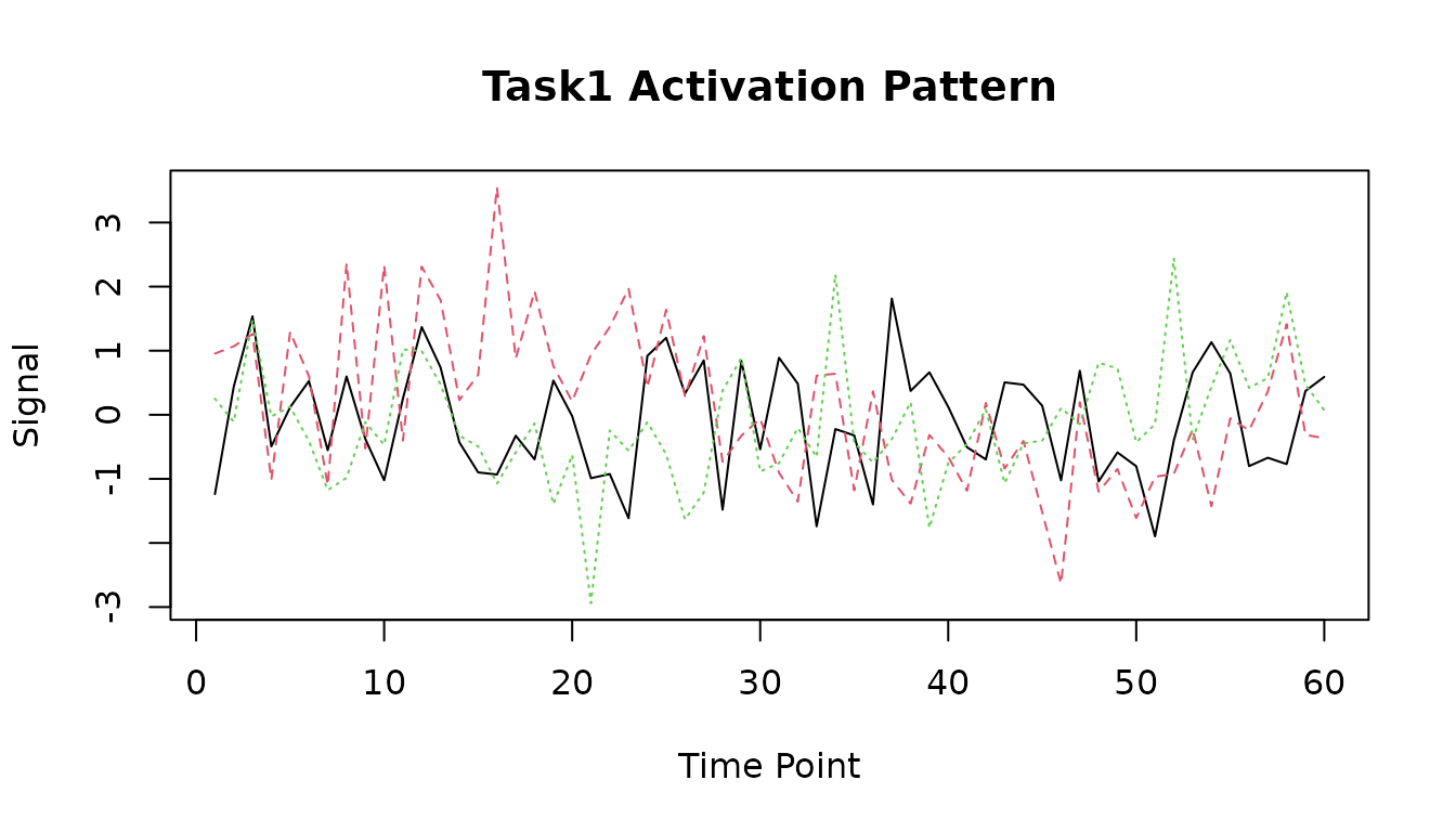
# Extract data from a specific run
task1_run <- multi_experiment@runs[["task1"]]
task1_data <- series(task1_run, i = 1:3) # First 3 voxels

# Show the activation pattern we added to task1
matplot(task1_data,
  type = "l",
  main = "Task1 Activation Pattern",
  xlab = "Time Point", ylab = "Signal"
)

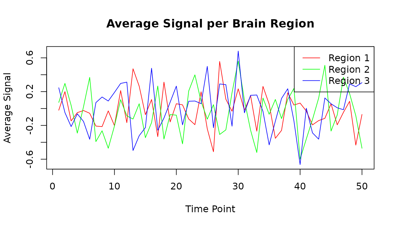
Creating Summary Data

# Sometimes you only need averaged data per region, not individual voxels
# The new interface makes this easy with the 'summary' parameter
summary_file <- tempfile(fileext = ".h5")

# Save just the cluster averages (much more compact)
write_dataset(runs_data[[1]], # Use the first run
  file = summary_file,
  clusters = clusters,
  summary = TRUE, # This is the key parameter
  scan_name = "rest_summary"
)
#> Creating HDF5 file: /tmp/Rtmpk1VJ8c/file22da5e700e24.h5
#> Writing global structures (mask, clusters, header)...
#> Writing scan data...
#>   Writing scan: rest_summary (type: summary)

# Load and examine the summary data
summary_experiment <- read_dataset(summary_file)
#> Detected type 'H5ParcellatedMultiScan' in file: /tmp/Rtmpk1VJ8c/file22da5e700e24.h5
#> Clusters argument is NULL, attempting to read from HDF5 file (/cluster_map).
summary_run <- summary_experiment@runs[[1]]

# This gives us a much smaller matrix (time × clusters instead of time × voxels)
summary_matrix <- as.matrix(summary_run)
cat("Summary data dimensions:", paste(dim(summary_matrix), collapse = " × "), "\n")
#> Summary data dimensions: 50 × 3
cat("(rows = time points, columns = clusters)\n")
#> (rows = time points, columns = clusters)

# Plot the average signal from each cluster
matplot(summary_matrix,
  type = "l", lty = 1,
  col = c("red", "green", "blue"),
  main = "Average Signal per Brain Region",
  xlab = "Time Point", ylab = "Average Signal"
)
legend("topright",
  legend = paste("Region", 1:3),
  col = c("red", "green", "blue"), lty = 1
)

Key Functions Summary

The new simplified interface provides three main functions:

`write_dataset()` - Save Your Data

# Basic usage - save one fMRI run with clusters
write_dataset(my_neurovec, file = "data.h5", clusters = my_clusters)

# Save multiple runs at once
write_dataset(list_of_neurovecs,
  file = "multi.h5", clusters = my_clusters,
  scan_names = c("run1", "run2", "run3")
)

# Save only cluster averages (more compact)
write_dataset(my_neurovec,
  file = "summary.h5", clusters = my_clusters,
  summary = TRUE
)

# Use median instead of mean for summaries
write_dataset(my_neurovec,
  file = "median.h5", clusters = my_clusters,
  summary = TRUE, summary_fun = median
)

`read_dataset()` - Load Your Data

# Automatic detection (recommended)
my_data <- read_dataset("data.h5")

# Specify type explicitly if needed
my_data <- read_dataset("data.h5", type = "H5ParcellatedMultiScan")

# Check what type a file contains
file_type <- detect_h5_type("mystery_file.h5")

`detect_h5_type()` - Identify File Contents

# Find out what's in an HDF5 file
detect_h5_type("my_file.h5")
# Returns: "H5ParcellatedMultiScan", "H5NeuroVec", "LatentNeuroVec", etc.

Memory Efficiency Tips

The H5ParcellatedMultiScan format is designed for efficiency:

# Compare file sizes
cat(
  "Original in-memory data size per run: ~",
  round(object.size(runs_data[[1]]) / 1024, 1), "KB\n"
)
#> Original in-memory data size per run: ~ 202.2 KB

cat(
  "HDF5 compressed file size: ",
  round(file.size(multi_file) / 1024, 1), "KB\n"
)
#> HDF5 compressed file size:  77.8 KB

cat(
  "Summary-only file size: ",
  round(file.size(summary_file) / 1024, 1), "KB\n"
)
#> Summary-only file size:  19.4 KB

# Memory usage when loading
cat(
  "\nMemory usage of loaded experiment object: ",
  format(object.size(multi_experiment), units = "KB"), "\n"
)
#> 
#> Memory usage of loaded experiment object:  87.7 Kb

# The actual data is loaded on-demand
small_extraction <- series(multi_experiment@runs[[1]], i = 1:2)
cat(
  "Memory usage of small data extraction: ",
  format(object.size(small_extraction), units = "KB"), "\n"
)
#> Memory usage of small data extraction:  1 Kb

When to Use H5ParcellatedMultiScan

✅ Good for: - Multi-run studies with consistent brain parcellation - ROI-based analyses - Large datasets that don’t fit in memory - Studies where you primarily analyze regional averages - Storing preprocessed data with known brain organization

❌ Not ideal for: - Single volumes (use H5NeuroVol) - Analyses requiring voxel-level flexibility across the whole brain - Data where the clustering might change between runs

Cleanup

# Always close HDF5 connections when done
close(experiment)
close(multi_experiment)
close(summary_experiment)

# Clean up temporary files
unlink(c(output_file, multi_file, summary_file))

Next Steps

For unclustered 4D data: See H5NeuroVec documentation
For dimensionality reduction: Explore LatentNeuroVec
For labeled brain regions: Check out LabeledVolumeSet
Package overview: Run help(package = "fmristore")

fmristore Package

2025-08-19

What is H5ParcellatedMultiScan?

Simple Example: From Data to Storage

Step 1: Create Brain Data

Step 2: Create Brain Regions (Clusters)

Step 3: Create Some fMRI Data

Step 4: Save Using the New Simple Interface

Step 5: Load Using the New Simple Interface

Step 6: Extract and Visualize Data

Advanced Example: Multiple Runs with Summary Data

Create Multiple Runs

Save Multiple Runs

Automatic Type Detection

Working with Multiple Runs

Creating Summary Data

Key Functions Summary

`write_dataset()` - Save Your Data

`read_dataset()` - Load Your Data

`detect_h5_type()` - Identify File Contents

Memory Efficiency Tips

When to Use H5ParcellatedMultiScan

Cleanup

Next Steps

Efficient Clustered fMRI Storage with H5ParcellatedMultiScan

fmristore Package

2025-08-19

What is H5ParcellatedMultiScan?

Simple Example: From Data to Storage

Step 1: Create Brain Data

Step 2: Create Brain Regions (Clusters)

Step 3: Create Some fMRI Data

Step 4: Save Using the New Simple Interface

Step 5: Load Using the New Simple Interface

Step 6: Extract and Visualize Data

Advanced Example: Multiple Runs with Summary Data

Create Multiple Runs

Save Multiple Runs

Automatic Type Detection

Working with Multiple Runs

Creating Summary Data

Key Functions Summary

write_dataset() - Save Your Data

read_dataset() - Load Your Data

detect_h5_type() - Identify File Contents

Memory Efficiency Tips

When to Use H5ParcellatedMultiScan

Cleanup

Next Steps

`write_dataset()` - Save Your Data

`read_dataset()` - Load Your Data

`detect_h5_type()` - Identify File Contents