Working with Individual Scans: H5ParcellatedScan and H5ParcellatedScanSummary

library(fmristore)
#> 
#> Attaching package: 'fmristore'
#> The following object is masked from 'package:stats':
#> 
#>     offset
library(neuroim2)
#> Loading required package: Matrix
#> 
#> Attaching package: 'neuroim2'
#> The following object is masked from 'package:base':
#> 
#>     scale

Overview: The Individual Scan Components

In the fmristore parcellated data system, H5ParcellatedMultiScan serves as a container that holds multiple individual scan objects. Each scan within the container is either:

H5ParcellatedScan: Full voxel-level time series data
H5ParcellatedScanSummary: Cluster-averaged time series data

This vignette focuses on working with these individual scan objects - how to access them from the parent H5ParcellatedMultiScan container and what operations you can perform on each scan type.

The Data Hierarchy

H5ParcellatedMultiScan (Container)
├── Run1 → H5ParcellatedScan (Full voxel data)
├── Run2 → H5ParcellatedScan (Full voxel data) 
├── Run3 → H5ParcellatedScanSummary (Cluster averages)
└── Run4 → H5ParcellatedScanSummary (Cluster averages)

Step 1: Create Sample Data Using the New Interface

First, let’s create a sample dataset using the modern write_dataset() and read_dataset() functions:

# Create a small brain with realistic structure
brain_dims <- c(10, 10, 5)
brain_space <- NeuroSpace(brain_dims, spacing = c(2, 2, 2))

# Define brain mask (central region)
mask_data <- array(FALSE, brain_dims)
mask_data[4:7, 4:7, 2:4] <- TRUE # Small brain region
mask <- LogicalNeuroVol(mask_data, brain_space)

# Divide brain into 3 clusters (regions)
n_voxels <- sum(mask)
cluster_assignments <- rep(1:3, length.out = n_voxels)
clusters <- ClusteredNeuroVol(mask, cluster_assignments)

cat("Created brain with", n_voxels, "voxels in", max(cluster_assignments), "clusters\n")
#> Created brain with 48 voxels in 3 clusters
print(table(clusters@clusters))
#> 
#>  1  2  3 
#> 16 16 16

Create Multiple fMRI Runs with Different Characteristics

# Create 3 different fMRI runs
run_names <- c("task_full", "rest_full", "task_summary")
runs_data <- list()

# Run 1: Task run (full data) - 60 timepoints
n_time1 <- 60
fmri_dims1 <- c(brain_dims, n_time1)
fmri_data1 <- array(rnorm(prod(fmri_dims1)), dim = fmri_dims1)

# Add task activation to cluster 2 (motor region)
cluster_2_voxels <- which(clusters@clusters == 2)
mask_indices <- which(mask, arr.ind = TRUE)
for (v in cluster_2_voxels) {
  x <- mask_indices[v, 1]
  y <- mask_indices[v, 2]
  z <- mask_indices[v, 3]
  # Add sinusoidal activation
  fmri_data1[x, y, z, ] <- fmri_data1[x, y, z, ] + 0.8 * sin(seq(0, 4 * pi, length.out = n_time1))
}

runs_data[[1]] <- NeuroVec(fmri_data1, NeuroSpace(fmri_dims1))

# Run 2: Rest run (full data) - 50 timepoints
n_time2 <- 50
fmri_dims2 <- c(brain_dims, n_time2)
fmri_data2 <- array(rnorm(prod(fmri_dims2)), dim = fmri_dims2)

# Add resting state connectivity pattern
for (i in 1:3) {
  cluster_voxels <- which(clusters@clusters == i)
  shared_signal <- rnorm(n_time2, sd = 0.3)
  for (v in cluster_voxels) {
    x <- mask_indices[v, 1]
    y <- mask_indices[v, 2]
    z <- mask_indices[v, 3]
    fmri_data2[x, y, z, ] <- fmri_data2[x, y, z, ] + shared_signal
  }
}

runs_data[[2]] <- NeuroVec(fmri_data2, NeuroSpace(fmri_dims2))

# Run 3: Will be saved as summary data (we'll use run 1's data)
runs_data[[3]] <- runs_data[[1]]

cat(
  "Created", length(runs_data), "runs with timepoints:",
  paste(sapply(runs_data, function(x) dim(x)[4]), collapse = ", "), "\n"
)
#> Created 3 runs with timepoints: 60, 50, 60

Save Mixed Full and Summary Data

# Save to HDF5 file - mix of full and summary scans
h5_file <- tempfile(fileext = ".h5")

# First, save the two full runs
write_dataset(list(runs_data[[1]], runs_data[[2]]),
  file = h5_file,
  clusters = clusters,
  scan_names = c("task_full", "rest_full"),
  summary = FALSE
) # Full voxel data
#> Creating HDF5 file: /tmp/RtmpasnhTW/file2318413d5c87.h5
#> Writing global structures (mask, clusters, header)...
#> Writing scan data...
#>   Writing scan: task_full (type: full)
#>     Scan 'task_full': nTime not in metadata, attempting to infer from sdata list.
#>     Scan 'task_full': Inferred nTime 60 from sdata item 'cluster_1'.
#>   Writing scan: rest_full (type: full)
#>     Scan 'rest_full': nTime not in metadata, attempting to infer from sdata list.
#>     Scan 'rest_full': Inferred nTime 50 from sdata item 'cluster_1'.

# Then add a summary run to the same file
# Note: In practice, you'd append this or use write_clustered_experiment_h5()
# For this example, we'll create separate files to show both types clearly

summary_file <- tempfile(fileext = ".h5")
write_dataset(runs_data[[3]],
  file = summary_file,
  clusters = clusters,
  scan_names = "task_summary",
  summary = TRUE
) # Cluster averages only
#> Creating HDF5 file: /tmp/RtmpasnhTW/file23181c1ab41e.h5
#> Writing global structures (mask, clusters, header)...
#> Writing scan data...
#>   Writing scan: scan_001 (type: summary)

cat("Created files:\n")
#> Created files:
cat("  Full data file:", round(file.size(h5_file) / 1024, 1), "KB\n")
#>   Full data file: 55 KB
cat("  Summary data file:", round(file.size(summary_file) / 1024, 1), "KB\n")
#>   Summary data file: 20.1 KB

Step 2: Load the Data with read_dataset()

# Load the datasets using the new read_dataset() function
full_experiment <- read_dataset(h5_file)
#> Detected type 'H5ParcellatedMultiScan' in file: /tmp/RtmpasnhTW/file2318413d5c87.h5
#> Clusters argument is NULL, attempting to read from HDF5 file (/cluster_map).
summary_experiment <- read_dataset(summary_file)
#> Detected type 'H5ParcellatedMultiScan' in file: /tmp/RtmpasnhTW/file23181c1ab41e.h5
#> Clusters argument is NULL, attempting to read from HDF5 file (/cluster_map).

cat("Full data experiment:\n")
#> Full data experiment:
print(full_experiment)
#> 
#> H5ParcellatedMultiScan
#>   # runs        : 2 
#>   # clusters    : 0 
#>   mask dims     : 10x10x5 
#>   HDF5 file     : /tmp/RtmpasnhTW/file2318413d5c87.h5
cat("\nSummary data experiment:\n")
#> 
#> Summary data experiment:
print(summary_experiment)
#> 
#> H5ParcellatedMultiScan
#>   # runs        : 1 
#>   # clusters    : 0 
#>   mask dims     : 10x10x5 
#>   HDF5 file     : /tmp/RtmpasnhTW/file23181c1ab41e.h5

Step 3: Accessing Individual Scans from the Container

This is the key concept: H5ParcellatedScan and H5ParcellatedScanSummary objects are accessed from their parent H5ParcellatedMultiScan container.

# Method 1: Access by position in @runs slot
task_scan <- full_experiment@runs[[1]] # First scan
rest_scan <- full_experiment@runs[[2]] # Second scan

# Method 2: Access by name if names are available
scan_names_full <- scan_names(full_experiment)
cat("Available scan names in full experiment:", paste(scan_names_full, collapse = ", "), "\n")
#> Available scan names in full experiment: rest_full, task_full

if (length(scan_names_full) > 0) {
  task_scan_by_name <- full_experiment@runs[[scan_names_full[1]]]
  cat("Accessed scan by name:", scan_names_full[1], "\n")
}
#> Accessed scan by name: rest_full

# Show what type of scan objects we got
cat("Task scan class:", class(task_scan), "\n")
#> Task scan class: H5ParcellatedScan
cat("Rest scan class:", class(rest_scan), "\n")
#> Rest scan class: H5ParcellatedScan

# Access the summary scan
summary_scan <- summary_experiment@runs[[1]]
cat("Summary scan class:", class(summary_scan), "\n")
#> Summary scan class: H5ParcellatedScanSummary

Understanding Individual Scan Properties

# Each individual scan has its own properties
cat("=== Task Scan (H5ParcellatedScan) ===\n")
#> === Task Scan (H5ParcellatedScan) ===
cat("Dimensions:", paste(dim(task_scan), collapse = " × "), "\n")
#> Dimensions: 10 × 10 × 5 × 50
cat("Class:", class(task_scan), "\n")
#> Class: H5ParcellatedScan
cat("Number of voxels:", dim(task_scan)[1], "\n")
#> Number of voxels: 10
cat("Number of timepoints:", dim(task_scan)[2], "\n\n")
#> Number of timepoints: 10

cat("=== Summary Scan (H5ParcellatedScanSummary) ===\n")
#> === Summary Scan (H5ParcellatedScanSummary) ===
summary_matrix <- as.matrix(summary_scan)
cat("Summary dimensions:", paste(dim(summary_matrix), collapse = " × "), "\n")
#> Summary dimensions: 60 × 3
cat("Class:", class(summary_scan), "\n")
#> Class: H5ParcellatedScanSummary
cat("Number of clusters:", ncol(summary_matrix), "\n")
#> Number of clusters: 3
cat("Number of timepoints:", nrow(summary_matrix), "\n\n")
#> Number of timepoints: 60

cat("=== Storage Efficiency ===\n")
#> === Storage Efficiency ===
n_voxels_full <- dim(task_scan)[1] * dim(task_scan)[2]
n_elements_summary <- prod(dim(summary_matrix))
cat("Full scan elements:", n_voxels_full, "\n")
#> Full scan elements: 100
cat("Summary scan elements:", n_elements_summary, "\n")
#> Summary scan elements: 180
cat("Compression ratio:", round(n_voxels_full / n_elements_summary, 1), ":1\n")
#> Compression ratio: 0.6 :1

H5ParcellatedScan: Operations on Individual Full Scans

When working with H5ParcellatedScan objects (full voxel data), you can extract time series for specific voxels and perform voxel-level analyses.

Extract Time Series from Individual Voxels

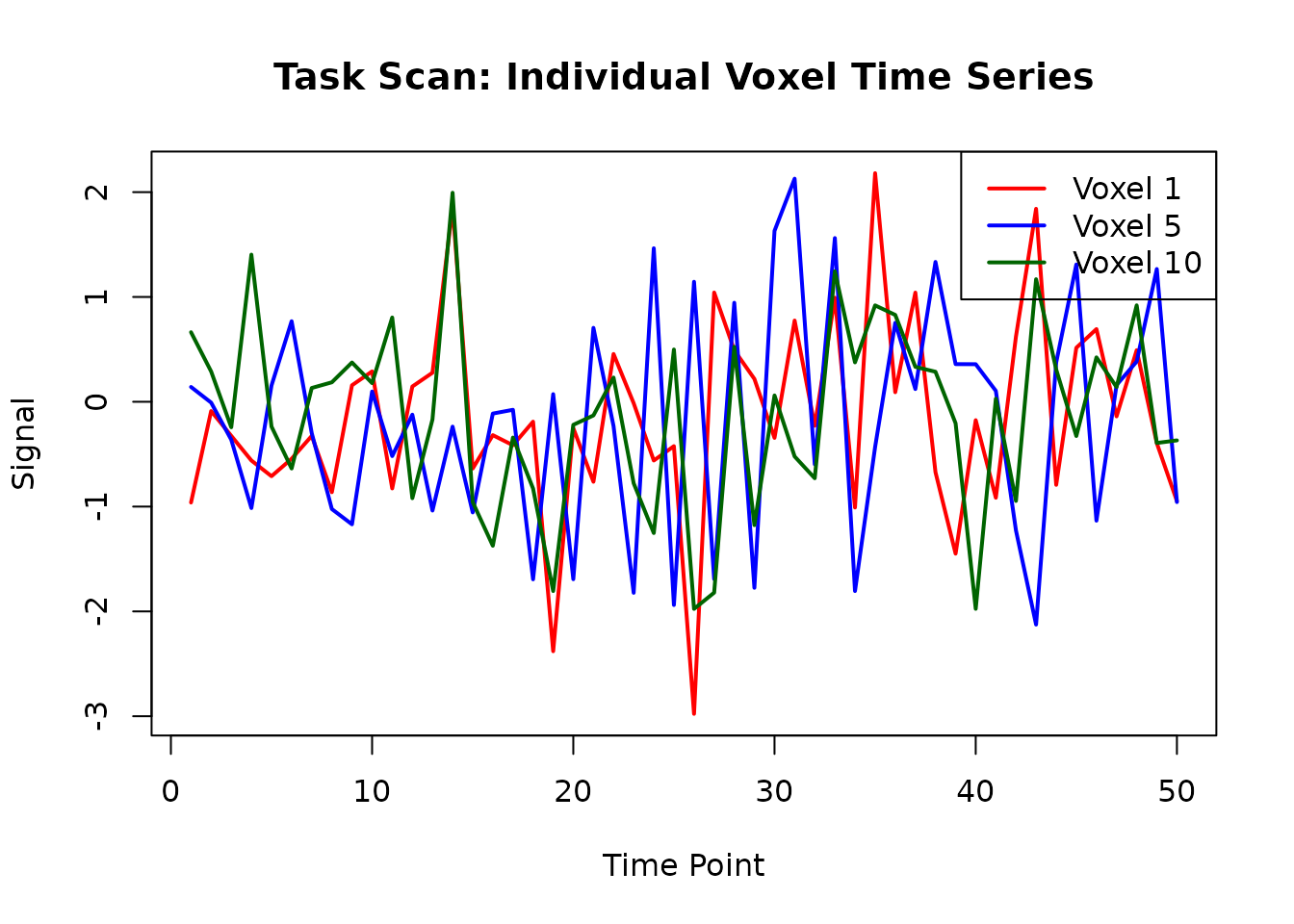
# Extract time series for specific voxel indices
voxel_indices <- c(1, 5, 10, 15)
task_voxel_ts <- series(task_scan, i = voxel_indices)

# Show what we extracted
cat("Extracted time series dimensions:", paste(dim(task_voxel_ts), collapse = " × "), "\n")
#> Extracted time series dimensions: 50 × 4
cat("(rows = timepoints, columns = voxels)\n\n")
#> (rows = timepoints, columns = voxels)

# Plot individual voxel time series
matplot(task_voxel_ts[, 1:3],
  type = "l", lty = 1, lwd = 2,
  main = "Task Scan: Individual Voxel Time Series",
  xlab = "Time Point", ylab = "Signal",
  col = c("red", "blue", "darkgreen")
)
legend("topright",
  legend = paste("Voxel", voxel_indices[1:3]),
  col = c("red", "blue", "darkgreen"), lty = 1, lwd = 2
)

Extract Time Series for All Voxels in a Cluster

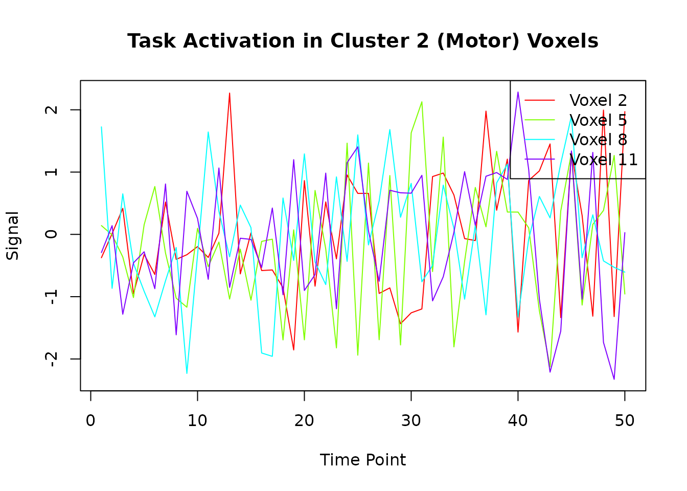
# Find all voxels in cluster 2 (the motor region with task activation)
cluster_2_voxels <- which(clusters@clusters == 2)
cat("Cluster 2 contains", length(cluster_2_voxels), "voxels\n")
#> Cluster 2 contains 16 voxels

# Extract time series for all voxels in cluster 2
cluster_2_ts <- series(task_scan, i = cluster_2_voxels)
cat("Cluster 2 time series dimensions:", paste(dim(cluster_2_ts), collapse = " × "), "\n")
#> Cluster 2 time series dimensions: 50 × 16

# Plot the first few voxels from cluster 2 to see the task activation
matplot(cluster_2_ts[, 1:min(4, ncol(cluster_2_ts))],
  type = "l", lty = 1,
  main = "Task Activation in Cluster 2 (Motor) Voxels",
  xlab = "Time Point", ylab = "Signal",
  col = rainbow(min(4, ncol(cluster_2_ts)))
)
legend("topright",
  legend = paste("Voxel", cluster_2_voxels[1:min(4, ncol(cluster_2_ts))]),
  col = rainbow(min(4, ncol(cluster_2_ts))), lty = 1
)

Compare Task vs Rest Scans (Individual Scan Analysis)

# Extract the same voxel indices from both scans
task_sample <- series(task_scan, i = 1:6)
rest_sample <- series(rest_scan, i = 1:6)

# Calculate variance for each voxel in each scan
task_vars <- apply(task_sample, 2, var)
rest_vars <- apply(rest_sample, 2, var)

# Compare
comparison_df <- data.frame(
  Voxel = 1:6,
  Task_Variance = task_vars,
  Rest_Variance = rest_vars,
  Ratio = task_vars / rest_vars
)

print("Variance comparison between task and rest scans:")
#> [1] "Variance comparison between task and rest scans:"
print(round(comparison_df, 3))
#>   Voxel Task_Variance Rest_Variance Ratio
#> 1     1         0.874         1.048 0.834
#> 2     2         1.067         1.559 0.684
#> 3     3         1.459         0.771 1.892
#> 4     4         0.801         0.729 1.099
#> 5     5         1.163         1.294 0.899
#> 6     6         1.050         1.095 0.958

# Plot comparison
par(mfrow = c(1, 2))
plot(task_vars, rest_vars,
  xlab = "Task Variance", ylab = "Rest Variance",
  main = "Variance Comparison", pch = 19, col = "blue"
)
abline(0, 1, col = "red", lty = 2)

plot(1:6, comparison_df$Ratio,
  type = "b", pch = 19, col = "darkgreen",
  xlab = "Voxel Index", ylab = "Task/Rest Variance Ratio",
  main = "Variance Ratio (Task/Rest)"
)
abline(h = 1, col = "red", lty = 2)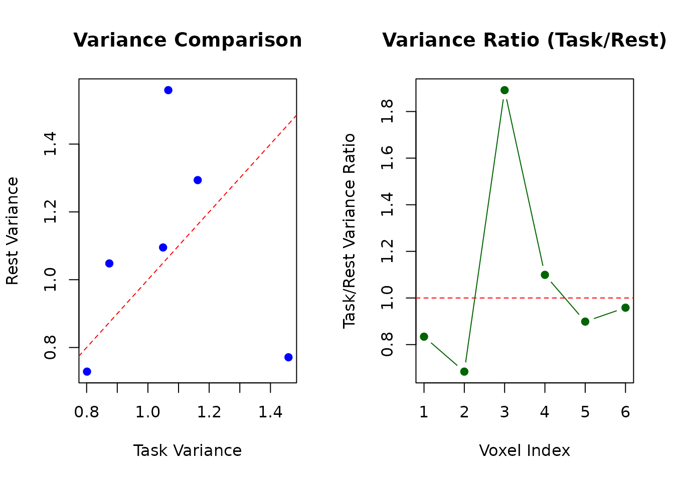

par(mfrow = c(1, 1))

H5ParcellatedScanSummary: Operations on Individual Summary Scans

When working with H5ParcellatedScanSummary objects, you work with cluster-averaged data that’s much more compact.

Extract and Analyze Summary Data

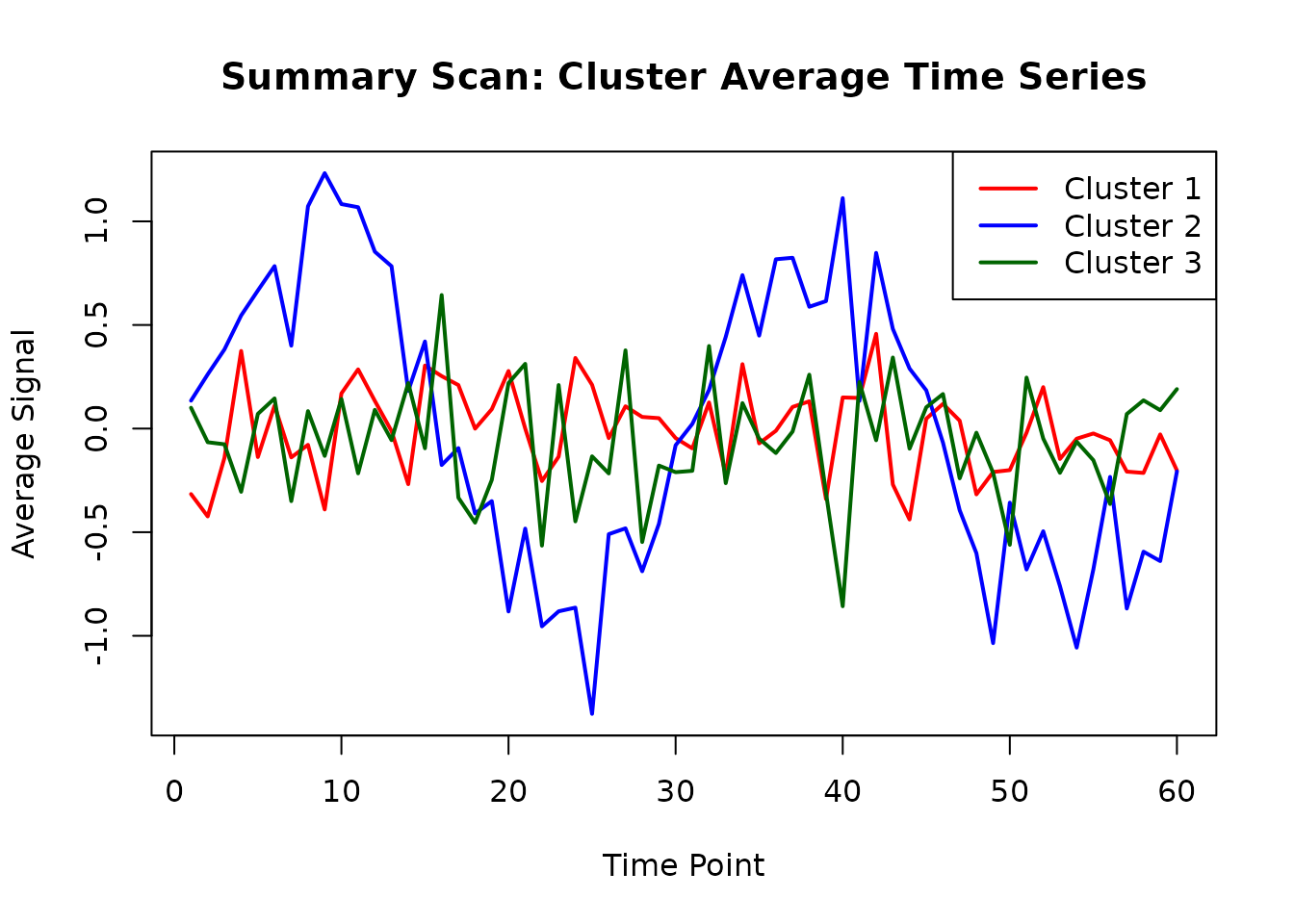
# Get the summary matrix (time × clusters)
summary_matrix <- as.matrix(summary_scan)
cat("Summary matrix dimensions:", paste(dim(summary_matrix), collapse = " × "), "\n")
#> Summary matrix dimensions: 60 × 3
cat("Timepoints:", nrow(summary_matrix), ", Clusters:", ncol(summary_matrix), "\n\n")
#> Timepoints: 60 , Clusters: 3

# Show column names if available
if (!is.null(colnames(summary_matrix))) {
  cat("Cluster names:", paste(colnames(summary_matrix), collapse = ", "), "\n")
} else {
  cat("Using default cluster numbering: 1 to", ncol(summary_matrix), "\n")
}
#> Cluster names: Cluster1, Cluster2, Cluster3

# Plot cluster averages over time
matplot(summary_matrix,
  type = "l", lty = 1, lwd = 2,
  main = "Summary Scan: Cluster Average Time Series",
  xlab = "Time Point", ylab = "Average Signal",
  col = c("red", "blue", "darkgreen")
)
legend("topright",
  legend = paste("Cluster", 1:ncol(summary_matrix)),
  col = c("red", "blue", "darkgreen"), lty = 1, lwd = 2
)

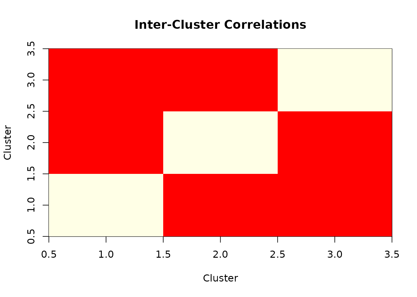
Compute Cluster-to-Cluster Correlations

# Calculate correlation matrix between clusters
cluster_correlations <- cor(summary_matrix)
cat("Cluster correlation matrix:\n")
#> Cluster correlation matrix:
print(round(cluster_correlations, 3))
#>          Cluster1 Cluster2 Cluster3
#> Cluster1    1.000    0.086    0.059
#> Cluster2    0.086    1.000    0.047
#> Cluster3    0.059    0.047    1.000

# Visualize correlation matrix
if (requireNamespace("corrplot", quietly = TRUE)) {
  corrplot::corrplot(cluster_correlations,
    method = "color",
    title = "Inter-Cluster Correlations",
    mar = c(0, 0, 2, 0)
  )
} else {
  # Simple heatmap alternative
  image(1:ncol(cluster_correlations), 1:nrow(cluster_correlations),
    as.matrix(cluster_correlations),
    main = "Inter-Cluster Correlations",
    xlab = "Cluster", ylab = "Cluster",
    col = heat.colors(20)
  )
}

Practical Usage Guidelines

Choose H5ParcellatedScan when you need:

Individual voxel analysis within clusters:

# Example: Find the most variable voxel in each cluster
most_variable_voxels <- sapply(1:3, function(cluster_id) {
  cluster_voxels <- which(clusters@clusters == cluster_id)
  cluster_ts <- series(task_scan, i = cluster_voxels)
  variances <- apply(cluster_ts, 2, var)
  cluster_voxels[which.max(variances)]
})

Voxel-wise statistical analyses:

# Example: Correlate each voxel with a task regressor
task_regressor <- sin(seq(0, 4 * pi, length.out = dim(task_scan)[2]))
all_voxel_ts <- series(task_scan, i = 1:dim(task_scan)[1])
voxel_correlations <- cor(all_voxel_ts, task_regressor)

Spatial pattern analysis within regions:

# Example: Identify activation hotspots within a cluster
cluster_1_voxels <- which(clusters@clusters == 1)
cluster_1_ts <- series(task_scan, i = cluster_1_voxels)
cluster_1_activation <- rowMeans(abs(cluster_1_ts)) # Activation magnitude

Choose H5ParcellatedScanSummary when you need:

Network connectivity analysis:

# Already computed above - cluster correlation matrix
print("Inter-cluster connectivity strengths:")
#> [1] "Inter-cluster connectivity strengths:"
diag(cluster_correlations) <- NA # Remove self-correlations
print(round(cluster_correlations, 3))
#>          Cluster1 Cluster2 Cluster3
#> Cluster1       NA    0.086    0.059
#> Cluster2    0.086       NA    0.047
#> Cluster3    0.059    0.047       NA

Efficient group comparisons:

# Example: Compare average activation levels between conditions
# If you had multiple summary scans, you could do:
cluster_means <- colMeans(summary_matrix)
names(cluster_means) <- paste("Cluster", 1:length(cluster_means))
print("Average activation per cluster:")
#> [1] "Average activation per cluster:"
print(round(cluster_means, 3))
#> Cluster 1 Cluster 2 Cluster 3 
#>    -0.012     0.004    -0.058

Memory-efficient temporal analysis:

# Example: Analyze temporal dynamics at cluster level
cluster_peak_times <- apply(summary_matrix, 2, which.max)
names(cluster_peak_times) <- paste("Cluster", 1:length(cluster_peak_times))
print("Peak activation timepoints per cluster:")
#> [1] "Peak activation timepoints per cluster:"
print(cluster_peak_times)
#> Cluster 1 Cluster 2 Cluster 3 
#>        42         9        16

Working with Both Scan Types in Practice

When you have an H5ParcellatedMultiScan container with mixed scan types:

# Access different scan types from the same experiment
full_scan1 <- full_experiment@runs[["task_full"]] # H5ParcellatedScan
full_scan2 <- full_experiment@runs[["rest_full"]] # H5ParcellatedScan
summary_scan <- summary_experiment@runs[["task_summary"]] # H5ParcellatedScanSummary

# Use appropriate methods for each type
voxel_data <- series(full_scan1, i = 1:10) # Voxel time series
cluster_data <- as.matrix(summary_scan) # Cluster averages

# Cannot use series() on summary scans - this would error:
# bad_call <- series(summary_scan, i = 1:5)  # ERROR!

Key Individual Scan Operations Summary

Operation	H5ParcellatedScan	H5ParcellatedScanSummary
`series(scan, i = indices)`	✅ Extract voxel time series	❌ Not available
`as.matrix(scan)`	❌ Not available	✅ Get cluster × time matrix
`dim(scan)`	✅ [voxels, timepoints]	❌ Use `dim(as.matrix(scan))`
`scan[i, j, k, t]`	✅ 4D indexing	❌ Not available
Memory efficiency	Lower (full voxel data)	Higher (cluster averages only)

Memory and Performance Considerations

# Compare memory footprint of different scan types
cat("Memory usage comparison:\n")
#> Memory usage comparison:
cat("  Task scan object size:", format(object.size(task_scan), units = "KB"), "\n")
#>   Task scan object size: 28.4 Kb
cat("  Summary scan object size:", format(object.size(summary_scan), units = "KB"), "\n")
#>   Summary scan object size: 29 Kb
cat("  Summary matrix size:", format(object.size(summary_matrix), units = "KB"), "\n\n")
#>   Summary matrix size: 2.1 Kb

# File size comparison
cat("File size comparison:\n")
#> File size comparison:
cat("  Full data file:", round(file.size(h5_file) / 1024, 1), "KB\n")
#>   Full data file: 55 KB
cat("  Summary data file:", round(file.size(summary_file) / 1024, 1), "KB\n")
#>   Summary data file: 20.1 KB

Clean Up

# Always close HDF5 connections when done
close(full_experiment)
close(summary_experiment)

# Clean up temporary files
unlink(c(h5_file, summary_file))

Key Takeaways

Individual scan objects (H5ParcellatedScan and H5ParcellatedScanSummary) are accessed from H5ParcellatedMultiScan containers via @runs[[index]] or @runs[["name"]]
H5ParcellatedScan provides voxel-level access within clusters:
- Use series(scan, i = indices) for individual voxel time series
- Supports 4D indexing: scan[i, j, k, t]
- Essential for spatial pattern analysis and voxel-wise statistics
H5ParcellatedScanSummary provides efficient cluster-level analysis:
- Use as.matrix(scan) to get time × cluster matrix
- Perfect for connectivity analysis and group comparisons
- Much smaller memory footprint
Modern workflow uses read_dataset() and write_dataset() functions for simplified data I/O with automatic type detection
Choose the right scan type based on your analysis needs:
- Full scans for detailed within-cluster analysis
- Summary scans for between-cluster connectivity and efficiency

Next Steps

For container management: See vignette("H5ParcellatedMultiScan") for working with multiple runs
For data creation: Learn about the new write_dataset() interface for saving parcellated data
For advanced analysis: Explore mixed designs with both full and summary scans in the same container

fmristore Package

2025-08-19