Working with Multiple Brain Maps using LabeledVolumeSet
fmristore Package
2026-03-29
Source:vignettes/LabeledVolumeSet.Rmd
LabeledVolumeSet.RmdWhat is a LabeledVolumeSet?
Imagine you have multiple brain maps from different conditions,
contrasts, or subjects that you want to store together efficiently.
LabeledVolumeSet is designed exactly for this scenario.
It’s like having a filing cabinet where each drawer (label) contains a
complete 3D brain map.
Key benefits: - Organized: Each brain volume has a meaningful label - Efficient: All volumes stored in a single HDF5 file - Consistent: All volumes share the same brain mask - Easy Access: Retrieve volumes by name or index
Quick Example: Storing Statistical Maps
Let’s say you have t-statistic maps from different contrasts in your fMRI study:
Step 2: Create Brain Mask
# Create a brain mask (only analyze certain voxels)
brain_mask <- array(TRUE, dim = brain_dims)
brain_mask[1:3, 1:3, ] <- FALSE # Exclude corners

# Convert to neuroim2 objects
stat_maps <- NeuroVec(contrast_data, NeuroSpace(c(brain_dims, n_contrasts)))
mask <- LogicalNeuroVol(brain_mask, NeuroSpace(brain_dims))
Step 3: Save with Labels
# Define meaningful labels
contrast_names <- c("Faces_vs_Houses", "Words_vs_Nonwords", "Motion_vs_Static")

# Save as LabeledVolumeSet
h5_file <- tempfile(fileext = ".h5")
h5_handle <- write_labeled_vec(stat_maps, mask, contrast_names, file = h5_file)
h5_handle$close_all()
Step 4: Load and Access
# Load the labeled set
labeled_maps <- read_labeled_vec(h5_file)

# Access by name
faces_map <- labeled_maps[["Faces_vs_Houses"]]
print(paste("Faces contrast map dimensions:", paste(dim(faces_map), collapse = "x")))
#> [1] "Faces contrast map dimensions: 10x10x5"

# See all available maps
print("Available contrasts:")
#> [1] "Available contrasts:"
print(labels(labeled_maps))
#> [1] "Faces_vs_Houses"   "Words_vs_Nonwords" "Motion_vs_Static"

close(labeled_maps)
unlink(h5_file)
Real-World Use Case: Group Analysis Results
Here’s how you might organize results from a group analysis:
# Simulate group analysis results
n_subjects <- 20
brain_dims <- c(20, 20, 10)
# Create different statistical maps
group_maps <- list(
mean_activation = array(rnorm(prod(brain_dims), mean = 0.5), brain_dims),
t_statistic = array(rt(prod(brain_dims), df = n_subjects - 1), brain_dims),
effect_size = array(rnorm(prod(brain_dims), mean = 0, sd = 0.3), brain_dims),
p_values = array(runif(prod(brain_dims)), brain_dims)
)
# Combine into a 4D array
all_maps <- array(unlist(group_maps), dim = c(brain_dims, length(group_maps)))
stat_vec <- NeuroVec(all_maps, NeuroSpace(c(brain_dims, length(group_maps))))
# Create a mask (e.g., only gray matter)
mask_array <- array(runif(prod(brain_dims)) > 0.3, brain_dims)
mask <- LogicalNeuroVol(mask_array, NeuroSpace(brain_dims))
# Save with descriptive labels
h5_file <- tempfile(fileext = ".h5")
h5_handle <- write_labeled_vec(stat_vec, mask, names(group_maps), file = h5_file)
h5_handle$close_all()
# Load and analyze
results <- read_labeled_vec(h5_file)
# Find significant voxels
p_map <- results[["p_values"]]
t_map <- results[["t_statistic"]]
# Threshold at p < 0.05
significant_voxels <- p_map < 0.05
n_sig <- sum(significant_voxels)
print(paste("Found", n_sig, "significant voxels"))
#> [1] "Found 1341 significant voxels"
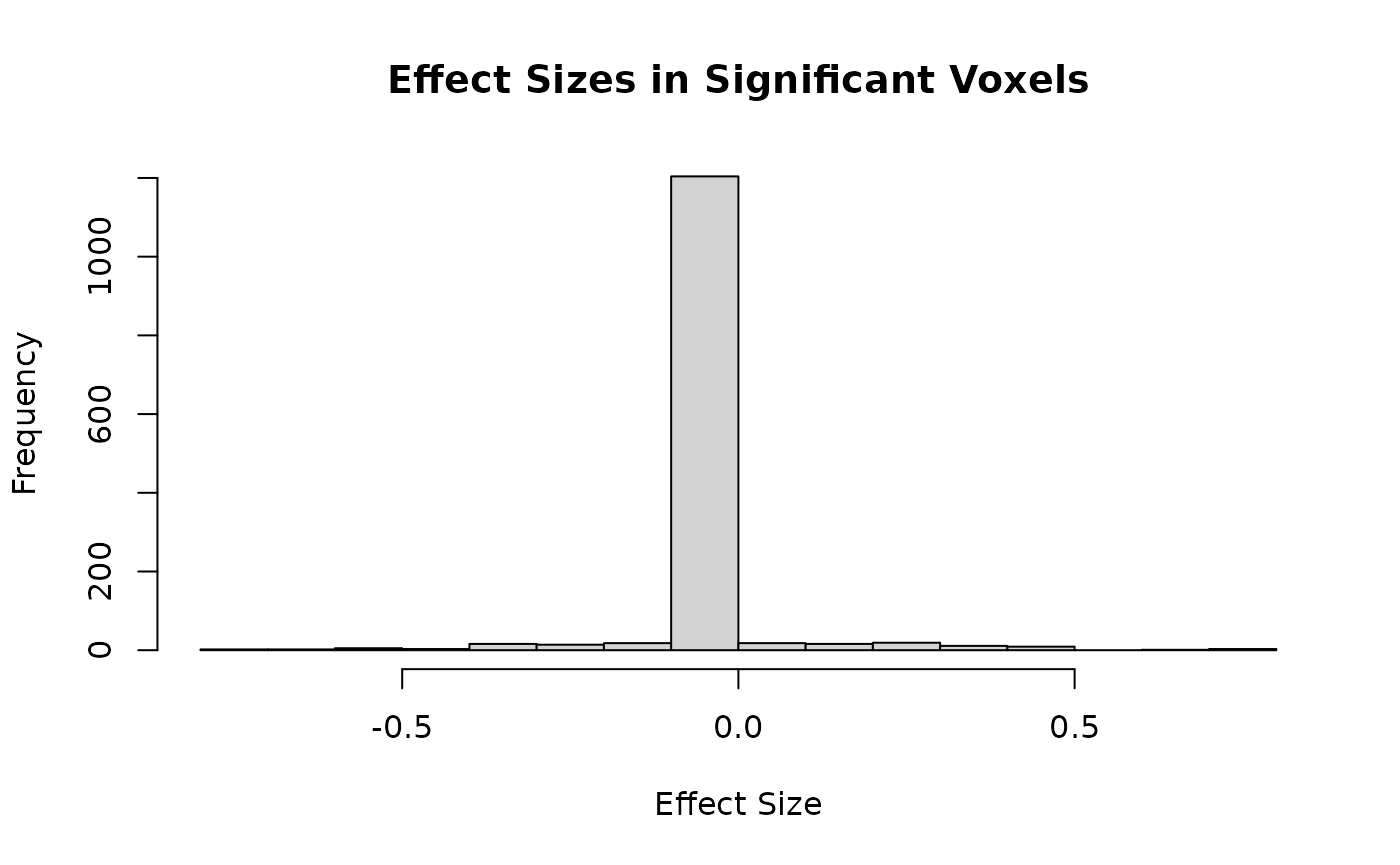
# Get effect sizes for significant voxels
if (n_sig > 0) {
effect_map <- results[["effect_size"]]
sig_effects <- effect_map[which(significant_voxels)]
hist(sig_effects,
main = "Effect Sizes in Significant Voxels",
xlab = "Effect Size"
)
}
Working with Subject-Specific Maps
Store individual subject maps for later analysis:
Add Activation Patterns
# Add subject-specific patterns
for (subj in 1:n_subjects) {
  # Each subject has slightly different activation center
  x_center <- 7 + subj
  y_center <- 7 + subj
  z_center <- 4

  # Add activation blob
  for (x in (x_center - 2):(x_center + 2)) {
    for (y in (y_center - 2):(y_center + 2)) {
      if (x > 0 && x <= brain_dims[1] && y > 0 && y <= brain_dims[2]) {
        subject_data[x, y, z_center, subj] <-
          subject_data[x, y, z_center, subj] + rnorm(1, mean = 3, sd = 0.5)
      }
    }
  }
}
Save Subject Maps
# Create objects
subject_vec <- NeuroVec(subject_data, NeuroSpace(c(brain_dims, n_subjects)))
mask <- LogicalNeuroVol(array(TRUE, brain_dims), NeuroSpace(brain_dims))
subject_labels <- paste0("Subject_", sprintf("%02d", 1:n_subjects))

# Save
h5_file <- tempfile(fileext = ".h5")
h5_handle <- write_labeled_vec(subject_vec, mask, subject_labels, file = h5_file)
h5_handle$close_all()
Compute Group Statistics
# Load and compute group average
subjects <- read_labeled_vec(h5_file)

# Extract all subjects' data efficiently
all_subjects_data <- subjects[, , , ] # Get all volumes at once

# Compute mean across subjects (4th dimension)
group_mean <- apply(all_subjects_data, c(1, 2, 3), mean)
print(paste("Group mean map dimensions:", paste(dim(group_mean), collapse = "x")))
#> [1] "Group mean map dimensions: 15x15x8"

# Find peak activation
peak_loc <- which(group_mean == max(group_mean), arr.ind = TRUE)
print(paste(
  "Peak activation at voxel:",
  paste(peak_loc, collapse = ", ")
))
#> [1] "Peak activation at voxel: 11, 9, 4"

close(subjects)
unlink(h5_file)
Advanced: Efficient Access Patterns
When working with many volumes, access them efficiently:
# Create a dataset with many conditions
n_conditions <- 10
brain_dims <- c(20, 20, 10)
condition_data <- array(rnorm(prod(brain_dims) * n_conditions),
dim = c(brain_dims, n_conditions)
)
condition_vec <- NeuroVec(condition_data, NeuroSpace(c(brain_dims, n_conditions)))
mask <- LogicalNeuroVol(array(TRUE, brain_dims), NeuroSpace(brain_dims))
condition_names <- paste0("Condition_", LETTERS[1:n_conditions])
h5_file <- tempfile(fileext = ".h5")
h5_handle <- write_labeled_vec(condition_vec, mask, condition_names, file = h5_file)
h5_handle$close_all()
# Load the dataset
conditions <- read_labeled_vec(h5_file)
# Method 1: Access specific conditions by name
print("Method 1: Individual access")
#> [1] "Method 1: Individual access"
cond_A <- conditions[["Condition_A"]]
cond_B <- conditions[["Condition_B"]]
# Method 2: Access multiple conditions at once
print("Method 2: Multiple conditions via indices")
#> [1] "Method 2: Multiple conditions via indices"
first_three <- conditions[, , , 1:3] # Get first 3 conditions
print(paste(
"Dimensions of first 3 conditions:",
paste(dim(first_three), collapse = "x")
))
#> [1] "Dimensions of first 3 conditions: 20x20x10x3"
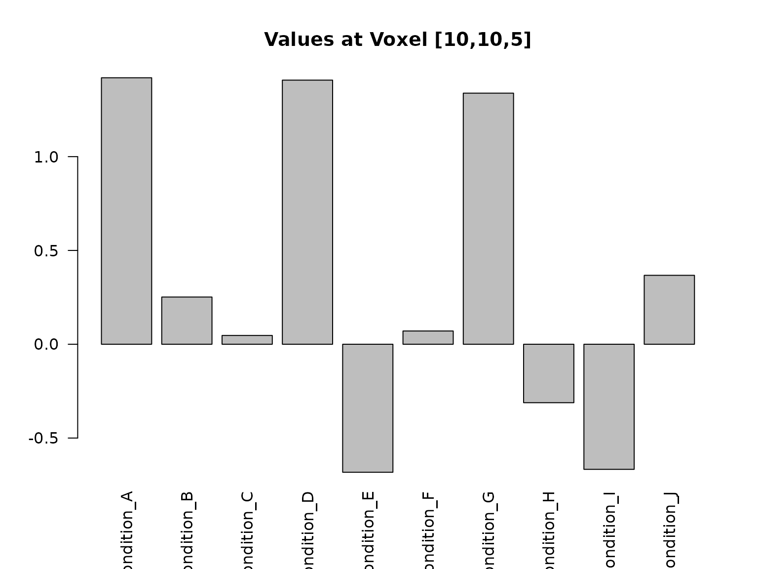
# Method 3: Extract values at specific voxel across all conditions
print("Method 3: Voxel time series across conditions")
#> [1] "Method 3: Voxel time series across conditions"
voxel_10_10_5 <- conditions[10, 10, 5, ]
barplot(voxel_10_10_5,
names.arg = condition_names,
las = 2, main = "Values at Voxel [10,10,5]"
)
Best Practices
2. Organize Your Analysis
# Save different analysis stages
write_labeled_vec(raw_maps, mask,
  paste0("Raw_", condition_names),
  file = "raw_maps.h5"
)

write_labeled_vec(smoothed_maps, mask,
  paste0("Smoothed_", condition_names),
  file = "smoothed_maps.h5"
)

write_labeled_vec(stats_maps, mask,
  paste0("Stats_", condition_names),
  file = "statistical_maps.h5"
)
3. Remember to Close
lvs <- read_labeled_vec("my_maps.h5")
# ... analysis code ...
close(lvs) # Always close when done!
Summary
LabeledVolumeSet makes it easy to: - Store multiple
related brain maps together - Access them by meaningful names - Work
efficiently with large collections - Keep your neuroimaging data
organized
Perfect for storing statistical maps, contrast images, subject data, or any collection of related 3D brain volumes!