Group Analysis

Bradley R. Buchsbaum

2026-04-03

library(fmrireg)
library(ggplot2)
set.seed(123)

Overview

This vignette walks through a compact, end-to-end example of group analysis with fmrireg. We first construct a small ROI-level dataset to illustrate the basic meta-regression interface, and then move to a voxelwise example using tiny synthetic NIfTI files. Along the way we show how to compare groups with fixed- and random-effects meta-analysis, how to obtain exact contrasts either at fit-time or post-hoc by saving covariance, and how to perform group inference from t-maps alone using Stouffer, Fisher, or Lancaster combinations.

Create a small ROI dataset

We simulate 10 subjects across two groups (A/B) for a single ROI. Group B has an effect that is 1 unit larger than group A. All subjects have the same SE for clarity.

n_per_group <- 5
subjects <- sprintf("s%02d", 1:(2 * n_per_group))
group <- factor(rep(c("A", "B"), each = n_per_group))

beta <- ifelse(group == "A", 0.5, 1.5)
se <- rep(0.25, length(beta))

roi_df <- data.frame(
  subject = subjects,
  roi = "ExampleROI",
  beta = beta,
  se = se,
  group = group,
  stringsAsFactors = FALSE
)

gd <- group_data_from_csv(
  roi_df,
  effect_cols = c(beta = "beta", se = "se"),
  subject_col = "subject",
  roi_col = "roi",
  covariate_cols = c("group")
)

gd
#> Group Data Object
#> Format: csv 
#> Subjects: 10 
#> Covariates: group

Fit group meta-analysis

We first fit an intercept-only model, then a model including a group term.

fit_fe <- fmri_meta(gd, formula = ~ 1, method = "fe", verbose = FALSE)

fit_cov <- fmri_meta(gd, formula = ~ 1 + group, method = "fe", verbose = FALSE)

print(fit_cov)
#> fMRI Meta-Analysis Results
#> ==========================
#> 
#> Method: fe 
#> Robust: none 
#> Formula: ~1 + group 
#> Subjects: 10 
#> ROIs analyzed: 1 
#> 
#> Heterogeneity:
#>   Mean tau^2: 0 
#>   Mean I^2: NaN %
summary(fit_cov)
#> fMRI Meta-Analysis Summary
#> ==========================
#> 
#> fMRI Meta-Analysis Results
#> ==========================
#> 
#> Method: fe 
#> Robust: none 
#> Formula: ~1 + group 
#> Subjects: 10 
#> ROIs analyzed: 1 
#> 
#> Heterogeneity:
#>   Mean tau^2: 0 
#>   Mean I^2: NaN %
#> 
#> Coefficients:
#>   (Intercept):
#>     Mean effect: 0.5 
#>     Mean SE: 0.1118034 
#>     Significant:1/1 (100%)
#>   groupB:
#>     Mean effect: 1 
#>     Mean SE: 0.1581139 
#>     Significant:1/1 (100%)

Note: With equal SE per subject, fixed-effects and random-effects will yield similar point estimates. Random-effects (method = "pm") will estimate between- subject heterogeneity (tau2) when present.

fit_pm <- fmri_meta(gd, formula = ~ 1 + group, method = "pm", verbose = FALSE)
summary(fit_pm)
#> fMRI Meta-Analysis Summary
#> ==========================
#> 
#> fMRI Meta-Analysis Results
#> ==========================
#> 
#> Method: pm 
#> Robust: none 
#> Formula: ~1 + group 
#> Subjects: 10 
#> ROIs analyzed: 1 
#> 
#> Heterogeneity:
#>   Mean tau^2: 0 
#>   Mean I^2: NaN %
#> 
#> Coefficients:
#>   (Intercept):
#>     Mean effect: 0.5 
#>     Mean SE: 0.1118034 
#>     Significant:1/1 (100%)
#>   groupB:
#>     Mean effect: 1 
#>     Mean SE: 0.1581139 
#>     Significant:1/1 (100%)

Extract coefficients and a contrast

coef_names <- colnames(fit_cov$coefficients)
coef_names
#> [1] "(Intercept)" "groupB"

coef_est <- as.numeric(fit_cov$coefficients[1, ])
names(coef_est) <- coef_names
coef_est
#> (Intercept)      groupB 
#>         0.5         1.0

if (any(grepl("group", coef_names))) {
  w <- rep(0, length(coef_names)); names(w) <- coef_names
  w[grep("group", coef_names)] <- 1
  con <- contrast(fit_cov, w)
  con
}
#> $estimate
#> [1] 1
#> 
#> $se
#> [1] 0.1581139
#> 
#> $z
#> [1] 6.324555
#> 
#> $p
#>                    [,1]
#> ExampleROI 2.539629e-10
#> 
#> $weights
#> (Intercept)      groupB 
#>           0           1 
#> 
#> $name
#> [1] "groupB"
#> 
#> $parent
#> fMRI Meta-Analysis Results
#> ==========================
#> 
#> Method: fe 
#> Robust: none 
#> Formula: ~1 + group 
#> Subjects: 10 
#> ROIs analyzed: 1 
#> 
#> Heterogeneity:
#>   Mean tau^2: 0 
#>   Mean I^2: NaN %
#> 
#> attr(,"class")
#> [1] "fmri_meta_contrast"

A quick visualization

We can visualize the group effects and their 95% CIs for the ROI-level fit.

df_tidy <- tidy(fit_cov, conf.int = TRUE)
df_tidy
#> # A tibble: 2 × 10
#>   roi        term     estimate std.error statistic  p.value  tau2    I2 conf.low
#>   <chr>      <chr>       <dbl>     <dbl>     <dbl>    <dbl> <dbl> <dbl>    <dbl>
#> 1 ExampleROI (Interc…      0.5     0.112      4.47 7.74e- 6     0    NA    0.281
#> 2 ExampleROI groupB        1       0.158      6.32 2.54e-10     0    NA    0.690
#> # ℹ 1 more variable: conf.high <dbl>

ggplot(df_tidy, aes(x = term, y = estimate, ymin = conf.low, ymax = conf.high)) +
  geom_pointrange() +
  geom_hline(yintercept = 0, linetype = 2) +
  labs(title = "ROI-level group meta-analysis",
       x = "Term", y = "Estimate +/- 95% CI") +
  theme_minimal()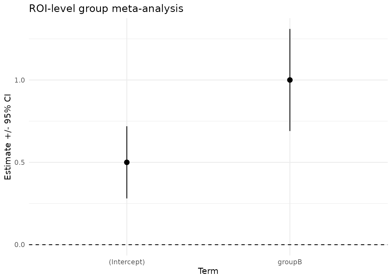

Notes on voxelwise analysis

For voxelwise analysis, construct group_data with format "nifti" or "h5":

# HDF5 (produced via write_results.fmri_lm)
# gd_h5 <- fmrireg::group_data(h5_paths, format = "h5",
#                     subjects = subject_ids,
#                     covariates = covariates_df,
#                     contrast = "ContrastName")

# NIfTI (provide per-subject paths for beta/SE or t)
# gd_nii <- fmrireg::group_data(list(beta = beta_paths, se = se_paths), format = "nifti",
#                      subjects = subject_ids,
#                      mask = "group_mask.nii.gz")

# fit <- fmri_meta(gd_h5, formula = ~ 1 + group, method = "pm")
# fit <- fmri_meta(gd_nii, formula = ~ 1, method = "fe")

For multiple comparisons correction that leverages spatial structure, see spatial_fdr() and create_3d_blocks().

Minimal NIfTI Example (Reproducible)

This chunk creates tiny synthetic NIfTI volumes on disk (in a temp dir) for a voxelwise demonstration. Group B has a higher effect in a small cube.

library(neuroim2)

set.seed(42)
tmpdir <- tempdir()
space <- NeuroSpace(c(8, 8, 8), spacing = c(2, 2, 2))

n_per_group <- 3
ids <- sprintf("sub-%02d", 1:(2 * n_per_group))
grp <- factor(rep(c("A", "B"), each = n_per_group))

active <- array(FALSE, dim = c(8, 8, 8))
active[3:5, 3:5, 3:5] <- TRUE

beta_paths <- character(length(ids))
se_paths   <- character(length(ids))

for (i in seq_along(ids)) {
  b <- array(0, dim = c(8, 8, 8))
  b[active] <- if (grp[i] == "A") 0.5 else 1.5
  b <- b + array(rnorm(length(b), sd = 0.05), dim = dim(b))
  v_beta <- NeuroVol(b, space)

  s <- array(0.25, dim = c(8, 8, 8))
  v_se <- NeuroVol(s, space)

  beta_paths[i] <- file.path(tmpdir, sprintf("%s_beta.nii.gz", ids[i]))
  se_paths[i]   <- file.path(tmpdir, sprintf("%s_se.nii.gz", ids[i]))
  write_vol(v_beta, beta_paths[i])
  write_vol(v_se,   se_paths[i])
}

mask_path <- file.path(tmpdir, "mask.nii.gz")
write_vol(NeuroVol(array(1, dim = c(8, 8, 8)), space), mask_path)

gd_nii <- group_data_from_nifti(
  beta_paths = beta_paths,
  se_paths   = se_paths,
  subjects   = ids,
  covariates = data.frame(group = grp),
  mask       = mask_path
)

fit_nii <- fmri_meta(gd_nii, formula = ~ 1 + group, method = "fe", verbose = FALSE)
fit_nii
#> fMRI Meta-Analysis Results
#> ==========================
#> 
#> Method: fe 
#> Robust: none 
#> Formula: ~1 + group 
#> Subjects: 6 
#> Voxels analyzed: 512 
#> 
#> Heterogeneity:
#>   Mean tau^2: 0 
#>   Mean I^2: 0 %

group_col <- grep("group", colnames(fit_nii$coefficients))
pvals <- 2 * pnorm(-abs(fit_nii$coefficients[, group_col] / fit_nii$se[, group_col]))
sum(pvals < 0.05)
#> [1] 27

sfr <- spatial_fdr(fit_nii, p = colnames(fit_nii$coefficients)[group_col], group = "blocks")
sum(sfr$reject)
#> [1] 75

img_group_est <- coef_image(fit_nii, colnames(fit_nii$coefficients)[group_col], statistic = "estimate")
range(as.array(img_group_est), na.rm = TRUE)
#> [1] -0.09585902  1.08515382

Exact contrasts and stored covariance

You can request exact contrasts at fit-time or store per-voxel covariance for exact post-hoc contrasts.

fit_nii_pm <- fmri_meta(
  gd_nii, formula = ~ 1 + group, method = "pm",
  return_cov = "tri", verbose = FALSE
)

con <- contrast(fit_nii_pm, c("(Intercept)" = 0, group = 1))
summary(con)
#>          Length Class     Mode     
#> estimate 512    -none-    numeric  
#> se       512    -none-    numeric  
#> z        512    -none-    numeric  
#> p        512    -none-    numeric  
#> weights    2    -none-    numeric  
#> name       1    -none-    character
#> parent    17    fmri_meta list

fit_nii_con <- fmri_meta(
  gd_nii, formula = ~ 1 + group, method = "pm",
  contrasts = matrix(c(0, 1), nrow = 1,
                     dimnames = list("group", colnames(fit_nii_pm$model$X))),
  verbose = FALSE
)
str(fit_nii_con$contrasts)
#> List of 4
#>  $ names   : chr "group"
#>  $ estimate: num [1:512, 1] 2.05e-02 1.79e-02 -3.49e-03 -5.51e-02 3.53e-05 ...
#>  $ se      : num [1:512, 1] 0.204 0.204 0.204 0.204 0.204 ...
#>  $ z       : num [1:512, 1] 0.100565 0.0878 -0.017112 -0.269929 0.000173 ...

Two-sample t-test (Welch and OLS) on NIfTI

As an alternative to meta-analysis, we can run two-sample voxelwise t-tests directly on the per-subject beta maps, using either Welch’s unequal-variance test or a standard OLS/Student t-test via a simple design matrix.

fit_welch <- fmri_ttest(gd_nii, formula = ~ 1 + group, engine = "welch")
t_welch   <- as.numeric(fit_welch$t["group", ])
df_welch  <- as.numeric(fit_welch$df["group", ])
p_welch   <- 2 * pt(abs(t_welch), df = df_welch, lower.tail = FALSE)

fit_ols   <- fmri_ttest(gd_nii, formula = ~ 1 + group, engine = "classic")
rn_t      <- rownames(fit_ols$t)
if (!is.null(rn_t) && any(rn_t == "group")) {
  t_ols <- fit_ols$t["group", ]
  df_ols <- as.numeric(fit_ols$df["group", ])
} else {
  t_ols <- fit_ols$t[2, ]
  df_ols <- rep(fit_ols$df[2, 1], length(t_ols))
}
p_ols    <- 2 * pt(abs(t_ols), df = df_ols, lower.tail = FALSE)

timg_welch <- NeuroVol(array(NA_real_, dim = c(8, 8, 8)), space)
mask_img   <- if (!is.null(gd_nii$mask_data)) gd_nii$mask_data else neuroim2::read_vol(mask_path)
timg_welch[as.array(mask_img) > 0] <- t_welch
range(as.array(timg_welch), na.rm = TRUE)
#> [1] -81.539233   4.582865

sum(p_welch < 0.05)
#> [1] 46
sum(p_ols   < 0.05)
#> [1] 51

Combining t-statistics only (Stouffer/Fisher/Lancaster)

When only per-subject t-statistics and degrees-of-freedom are available, you can still carry out group inference without betas/SEs by setting combine = in fmri_meta() (or in fmri_ttest(..., engine = "meta")). Stouffer combines signed z-scores and supports equal, inverse-variance or custom weights; Fisher combines p-values with equal weights; and Lancaster provides a weighted Fisher variant by mapping weights to per-subject degrees-of-freedom.

dat_full <- read_nifti_full(gd_nii)
tmat <- dat_full$beta / dat_full$se

t_paths <- character(length(ids))
for (i in seq_along(ids)) {
  img <- NeuroVol(array(NA_real_, dim = c(8, 8, 8)), space)
  img[as.array(neuroim2::read_vol(mask_path)) > 0] <- tmat[i, ]
  pth <- file.path(tmpdir, sprintf("%s_t.nii.gz", ids[i]))
  write_vol(img, pth)
  t_paths[i] <- pth
}

gd_t <- group_data_from_nifti(
  t_paths  = t_paths,
  df       = 60,
  subjects = ids,
  covariates = data.frame(group = grp),
  mask     = mask_path
)

fit_st <- fmri_meta(gd_t, formula = ~ 1, combine = "stouffer", verbose = FALSE)

w_subj <- rep(1, length(ids))
fit_st_w <- fmri_meta(gd_t, formula = ~ 1, combine = "stouffer",
                      weights = "custom", weights_custom = w_subj,
                      verbose = FALSE)

fit_fi  <- fmri_meta(gd_t, formula = ~ 1, combine = "fisher", verbose = FALSE)
fit_la  <- fmri_meta(gd_t, formula = ~ 1, combine = "lancaster",
                     weights = "custom", weights_custom = w_subj,
                     verbose = FALSE)

Meta engine via fmri_ttest with weights

The t-test interface supports the meta engine with equal/custom weighting.

fit_tt_meta <- fmri_ttest(gd_nii, formula = ~ 1 + group, engine = "meta",
                          weights = "equal")

w_subj <- rep(1, length(ids))
fit_tt_meta_w <- fmri_ttest(gd_nii, formula = ~ 1 + group, engine = "meta",
                            weights = "custom", weights_custom = w_subj)

fit_tt_la <- fmri_ttest(gd_t, formula = ~ 1, engine = "meta",
                        combine = "lancaster", weights = "custom",
                        weights_custom = w_subj)

ROI t-only example (Stouffer and Lancaster)

You can also combine t-statistics at the ROI level from a tabular CSV. Provide per-subject t and df, then choose a combine method.

roi_t_df <- data.frame(
  subject = subjects,
  roi = "ExampleROI",
  t = rnorm(length(subjects), mean = 2.0, sd = 0.5),
  df = 40,
  stringsAsFactors = FALSE
)

gd_roi_t <- group_data_from_csv(
  roi_t_df,
  effect_cols = c(t = "t", df = "df"),
  subject_col = "subject",
  roi_col = "roi"
)

fit_roi_st <- fmri_meta(gd_roi_t, formula = ~ 1, combine = "stouffer", verbose = FALSE)

w_roi <- rep(1, length(subjects))
fit_roi_la <- fmri_meta(gd_roi_t, formula = ~ 1, combine = "lancaster",
                        weights = "custom", weights_custom = w_roi,
                        verbose = FALSE)

c(fit_roi_st$method, fit_roi_la$method)
#> [1] "pm" "pm"

A brief recap

Meta-analysis in fmrireg supports fixed-effects and several random-effects estimators (method = "fe"|"pm"|"dl"|"reml"), with optional robust Huber weighting. You can pass subject-level covariates for group comparisons and, when working from t-maps only, set combine = to use Stouffer, Fisher, or Lancaster. Exact contrasts are available either at fit-time (via contrasts=) or post-hoc by saving packed covariance with return_cov = "tri" and then calling contrast(). Weighting applies to both meta-regression and t-only combinations (weights = "ivw"|"equal"|"custom", with weights_custom as a vector of length subjects or an S x P matrix). The examples above show ROI-based meta-regression, voxelwise fits from NIfTI, and t-only combinations via both fmri_meta() and fmri_ttest(..., engine = "meta").