Contrasts and Hypothesis Tests
Bradley R. Buchsbaum
2026-06-21
Source:vignettes/a_05_contrasts.Rmd
a_05_contrasts.RmdIntroduction to Contrasts
Statistical contrasts are a fundamental component of fMRI
analyses, allowing researchers to test specific hypotheses about
differences in brain activity between experimental conditions. The
fmrireg package provides a flexible and powerful system for
defining, computing, and applying contrasts to linear models fitted to
fMRI data.
This vignette explores the various ways to specify contrasts in
fmrireg, from simple pairwise comparisons to more complex
interactions and polynomial trends.
Example: A 2x2 Factorial Design
To illustrate the contrast functionalities, let’s use a simple two-by-two factorial design. We have two factors:
- category: with levels “face” and “scene”
- attention: with levels “attend” and “ignore”
We’ll assume each unique condition is repeated twice within a single run.
First, we construct the event table representing this design:
design <- expand.grid(category = c("face", "scene"),
                      attention = c("attend", "ignore"),
                      replication = c(1, 2))
design$onset <- seq(1, 100, length.out = nrow(design)) # Assign arbitrary onsets
design$block <- rep(1, nrow(design))                  # Single block (run)

# Ensure factors are factors
design$category <- factor(design$category)
design$attention <- factor(design$attention)

kable(design, caption = "2x2 Experimental Design Table")| category | attention | replication | onset | block |
|---|---|---|---|---|
| face | attend | 1 | 1.00000 | 1 |
| scene | attend | 1 | 15.14286 | 1 |
| face | ignore | 1 | 29.28571 | 1 |
| scene | ignore | 1 | 43.42857 | 1 |
| face | attend | 2 | 57.57143 | 1 |
| scene | attend | 2 | 71.71429 | 1 |
| face | ignore | 2 | 85.85714 | 1 |
| scene | ignore | 2 | 100.00000 | 1 |
# Define a sampling frame and create the event model
sframe <- sampling_frame(blocklens = 120, TR = 2)
emodel <- event_model(onset ~ hrf(category, attention),
                      block = ~block,
                      data = design,
                      sampling_frame = sframe)

# Extract the event term for contrast calculation
# In this simple model, there's only one event term
event_term <- terms(emodel)[[1]]

kable(cells(event_term), caption = "Cells within the 'category:attention' event term")| category | attention |
|---|---|
| face | attend |
| scene | attend |
| face | ignore |
| scene | ignore |
This event_term object encapsulates the structure of our
experimental conditions and will be used to compute contrast
weights.
Basic Contrasts: pair_contrast
The most common type of contrast compares the average activation of
one set of conditions against another. The pair_contrast
function provides a convenient way to define such sum-to-zero
contrasts.
Defining Pair Contrasts
pair_contrast takes two formulas, A and
B, defining the conditions to compare, and a mandatory
name.
Let’s define contrasts for the main effects of category (face vs. scene) and attention (attend vs. ignore):
# Main effect of category: face > scene
con_face_vs_scene <- pair_contrast(~ category == "face",
                                 ~ category == "scene",
                                 name = "face_vs_scene")

# Main effect of attention: attend > ignore
con_attend_vs_ignore <- pair_contrast(~ attention == "attend",
                                    ~ attention == "ignore",
                                    name = "attend_vs_ignore")
Computing Contrast Weights
Contrast specifications are abstract until applied to a specific
model term structure. The contrast_weights function
computes the numerical weights based on the levels within the term.
wts_face_vs_scene <- contrast_weights(con_face_vs_scene, event_term)
wts_attend_vs_ignore <- contrast_weights(con_attend_vs_ignore, event_term)

cat("Weights for 'face_vs_scene':\n")
#> Weights for 'face_vs_scene':
kable(wts_face_vs_scene$weights, col.names = wts_face_vs_scene$name)| face_vs_scene | |
|---|---|
| category.face_attention.attend | 0.5 |
| category.scene_attention.attend | -0.5 |
| category.face_attention.ignore | 0.5 |
| category.scene_attention.ignore | -0.5 |
cat("\nWeights for 'attend_vs_ignore':\n")
#>
#> Weights for 'attend_vs_ignore':
kable(wts_attend_vs_ignore$weights, col.names = wts_attend_vs_ignore$name)| attend_vs_ignore | |
|---|---|
| category.face_attention.attend | 0.5 |
| category.scene_attention.attend | 0.5 |
| category.face_attention.ignore | -0.5 |
| category.scene_attention.ignore | -0.5 |
Notice how pair_contrast automatically averages over the
levels not mentioned in the formulas. For
face_vs_scene, it averages over ‘attend’ and ‘ignore’
within each category level before contrasting. The resulting weights sum
to zero (0.25 * 2 + (-0.25) * 2 = 0).
Unit Contrasts: Comparing to Baseline
Sometimes, we want to test whether activation for a condition (or set
of conditions) is significantly different from the implicit baseline
(often represented by the intercept in the model).
unit_contrast is used for this purpose. It creates
contrasts that sum to 1.
con_face_vs_baseline <- unit_contrast(~ category == "face", name = "face_gt_baseline")
con_attend_vs_baseline <- unit_contrast(~ attention == "attend", name = "attend_gt_baseline")

wts_face_vs_baseline <- contrast_weights(con_face_vs_baseline, event_term)
wts_attend_vs_baseline <- contrast_weights(con_attend_vs_baseline, event_term)

cat("Weights for 'face_gt_baseline':\n")
#> Weights for 'face_gt_baseline':
kable(wts_face_vs_baseline$weights, col.names = wts_face_vs_baseline$name)| face_gt_baseline | |
|---|---|
| category.face_attention.attend | 0.25 |
| category.scene_attention.attend | 0.25 |
| category.face_attention.ignore | 0.25 |
| category.scene_attention.ignore | 0.25 |
cat("\nWeights for 'attend_gt_baseline':\n")
#>
#> Weights for 'attend_gt_baseline':
kable(wts_attend_vs_baseline$weights, col.names = wts_attend_vs_baseline$name)| attend_gt_baseline | |
|---|---|
| category.face_attention.attend | 0.25 |
| category.scene_attention.attend | 0.25 |
| category.face_attention.ignore | 0.25 |
| category.scene_attention.ignore | 0.25 |
These weights average the specified conditions and compare them against zero (the implicit baseline).
General Contrasts with contrast()
The contrast() function allows for more complex
contrasts defined by a single formula expression. This is useful for
interactions or specific linear combinations of conditions.
Let’s define the interaction contrast: (face:attend - face:ignore) - (scene:attend - scene:ignore). This tests if the effect of attention differs between categories.
# Interaction contrast
con_interaction <- contrast(
  ~ (`face:attend` - `face:ignore`) - (`scene:attend` - `scene:ignore`),
  name = "category_X_attention"
)

wts_interaction <- contrast_weights(con_interaction, event_term)

cat("Weights for 'category_X_attention':\n")
#> Weights for 'category_X_attention':
kable(wts_interaction$weights, col.names = wts_interaction$name)| category_X_attention | |
|---|---|
| category.face_attention.attend | 1 |
| category.scene_attention.attend | -1 |
| category.face_attention.ignore | -1 |
| category.scene_attention.ignore | 1 |
Note: In the formula for contrast(), condition names are
formed by joining factor levels with colons (e.g.,
face:attend). When condition names contain special
characters like colons, they must be enclosed in backticks. The
contrast_weights function evaluates this formula in an
environment where each condition name corresponds to a column vector (1
for that condition, 0 otherwise).
Contrasts for Main Effects and Interactions
While pair_contrast and contrast are
flexible, fmrireg provides convenience functions for
standard ANOVA-like contrasts.
-
oneway_contrast: Generates contrasts for the main effect of a single factor (sum-to-zero coding). -
interaction_contrast: Generates contrasts for interaction effects between two or more factors.
These often result in multiple contrast columns (F-contrasts) testing the overall effect.
# Main effect of category (will produce 1 contrast vector)
con_main_category <- oneway_contrast(~ category, name = "Main_Category")
wts_main_category <- contrast_weights(con_main_category, event_term)

# Interaction effect (will produce 1 contrast vector for a 2x2 design)
con_int_cat_att <- interaction_contrast(~ category * attention, name = "Interaction_CatAtt")
wts_int_cat_att <- contrast_weights(con_int_cat_att, event_term)

cat("Weights for 'Main_Category' (oneway_contrast):\n")
#> Weights for 'Main_Category' (oneway_contrast):
kable(wts_main_category$weights)| Main_Category_1 | |
|---|---|
| category.face_attention.attend | -1 |
| category.scene_attention.attend | 1 |
| category.face_attention.ignore | -1 |
| category.scene_attention.ignore | 1 |
cat("\nWeights for 'Interaction_CatAtt' (interaction_contrast):\n")
#>
#> Weights for 'Interaction_CatAtt' (interaction_contrast):
kable(wts_int_cat_att$weights)| Interaction_CatAtt_1 | |
|---|---|
| face_attend | 1 |
| scene_attend | -1 |
| face_ignore | -1 |
| scene_ignore | 1 |
Note that the weights generated by
interaction_contrast(~ category * attention) match those we
manually specified using contrast(). For factors with more
levels, these functions would generate multiple orthogonal contrast
columns.
Polynomial Contrasts for Ordered Factors
If a factor represents ordered levels (e.g., different task
difficulty levels, time points), poly_contrast can test for
trends (linear, quadratic, etc.).
Let’s add an ‘intensity’ factor to our design:
design_poly <- expand.grid(category = c("face", "scene"),
                           intensity = c(1, 2, 3), # Ordered factor
                           replication = c(1))
design_poly$onset <- seq(1, 60, length.out = nrow(design_poly))
design_poly$block <- rep(1, nrow(design_poly))
design_poly$intensity <- factor(design_poly$intensity, ordered = TRUE)

kable(design_poly, caption = "Design with Ordered 'intensity' Factor")| category | intensity | replication | onset | block |
|---|---|---|---|---|
| face | 1 | 1 | 1.0 | 1 |
| scene | 1 | 1 | 12.8 | 1 |
| face | 2 | 1 | 24.6 | 1 |
| scene | 2 | 1 | 36.4 | 1 |
| face | 3 | 1 | 48.2 | 1 |
| scene | 3 | 1 | 60.0 | 1 |
emodel_poly <- event_model(onset ~ hrf(category, intensity),
                           block = ~block,
                           data = design_poly,
                           sampling_frame = sframe)
event_term_poly <- terms(emodel_poly)[[1]]
Now, define a polynomial contrast to test for linear and quadratic trends of intensity:
con_poly_intensity <- poly_contrast(~ intensity, degree = 2, name = "Intensity_Trend")
wts_poly_intensity <- contrast_weights(con_poly_intensity, event_term_poly)

cat("Weights for 'Intensity_Trend' (poly_contrast, degree=2):\n")
#> Weights for 'Intensity_Trend' (poly_contrast, degree=2):
kable(wts_poly_intensity$weights)| Intensity_Trend_1 | Intensity_Trend_2 | |
|---|---|---|
| category.face_intensity.1 | -0.5 | 0.2886751 |
| category.scene_intensity.1 | -0.5 | 0.2886751 |
| category.face_intensity.2 | 0.0 | -0.5773503 |
| category.scene_intensity.2 | 0.0 | -0.5773503 |
| category.face_intensity.3 | 0.5 | 0.2886751 |
| category.scene_intensity.3 | 0.5 | 0.2886751 |
The output has two columns: poly1 for the linear trend
and poly2 for the quadratic trend.
Helper Functions for Common Comparisons
Two helpers simplify common multi-level comparisons:
-
pair_contrast: Creates a pairwise comparison between two levels of a factor. -
one_against_all_contrast: Compares each level against the average of all other levels.
# Pairwise contrast for category using pair_contrast
con_pairwise_cat <- pair_contrast(~ category == "face",
                                 ~ category == "scene",
                                 name = "cat_face_scene")

# Compare each attention level vs the other
con_one_all_att <- one_against_all_contrast(levels(design$attention), facname = "attention")

# Since con_one_all_att is already a contrast_set, we need to extract its elements
# and combine them properly with the single contrast
all_helper_contrasts <- list(con_pairwise_cat)
all_helper_contrasts <- append(all_helper_contrasts, con_one_all_att)
con_set_helpers <- do.call(contrast_set, all_helper_contrasts)

# Calculate weights (demonstrating contrast_set)
wts_helpers <- contrast_weights(con_set_helpers, event_term)

# Display weights for one_against_all
cat("Weights for 'con_attend_vs_other':\n")
#> Weights for 'con_attend_vs_other':
kable(wts_helpers$con_attend_vs_other$weights)| con_attend_vs_other | |
|---|---|
| category.face_attention.attend | 0.5 |
| category.scene_attention.attend | 0.5 |
| category.face_attention.ignore | -0.5 |
| category.scene_attention.ignore | -0.5 |
cat("\nWeights for 'con_ignore_vs_other':\n")
#>
#> Weights for 'con_ignore_vs_other':
kable(wts_helpers$con_ignore_vs_other$weights)| con_ignore_vs_other | |
|---|---|
| category.face_attention.attend | -0.5 |
| category.scene_attention.attend | -0.5 |
| category.face_attention.ignore | 0.5 |
| category.scene_attention.ignore | 0.5 |
Grouping Contrasts: contrast_set
You can group multiple contrast specifications using
contrast_set. When contrast_weights is called
on a contrast_set, it returns a named list of computed
contrast weight objects.
# Combine several previously defined contrasts
all_contrasts <- contrast_set(
  con_face_vs_scene,
  con_attend_vs_ignore,
  con_interaction,
  con_face_vs_baseline
)

print(all_contrasts)
#>
#> === Contrast Set ===
#>
#>  Overview:
#>   * Number of contrasts: 4
#>   * Types of contrasts:
#>     - contrast_formula_spec : 1
#>     - pair_contrast_spec : 2
#>     - unit_contrast_spec : 1
#>
#>   Individual Contrasts:
#>
#> [1] face_vs_scene (pair_contrast_spec)
#>     Formula: ~category == "face" vs  ~category == "scene"
#>
#> [2] attend_vs_ignore (pair_contrast_spec)
#>     Formula: ~attention == "attend" vs  ~attention == "ignore"
#>
#> [3] category_X_attention (contrast_formula_spec)
#>     Formula: ~(`face:attend` - `face:ignore`) - (`scene:attend` - `scene:ignore`)
#>
#> [4] face_gt_baseline (unit_contrast_spec)
#>     Formula: ~category == "face"

# Compute weights for the entire set
all_weights <- contrast_weights(all_contrasts, event_term)

# Access weights for a specific contrast within the set
cat("\nAccessing weights for 'face_vs_scene' from the set:\n")
#>
#> Accessing weights for 'face_vs_scene' from the set:
kable(all_weights$face_vs_scene$weights)| face_vs_scene | |
|---|---|
| category.face_attention.attend | 0.5 |
| category.scene_attention.attend | -0.5 |
| category.face_attention.ignore | 0.5 |
| category.scene_attention.ignore | -0.5 |
Applying Contrasts in fmri_lm
Contrasts are typically specified within the hrf()
function in the fmri_lm formula. You can provide a single
contrast specification or a contrast_set.
# Simulate some simple data for demonstration
ysim <- matrix(rnorm(120 * 3), 120, 3) # 3 voxels
dataset_sim <- matrix_dataset(ysim, TR = 2, run_length = 120, event_table = design)

# Fit model with the contrast set defined earlier
fmri_fit <- fmri_lm(
  formula = onset ~ hrf(category, attention, contrasts = all_contrasts),
  block = ~ block,
  dataset = dataset_sim,
  strategy = "chunkwise" # Use chunkwise for matrix_dataset
)

# Print summary of the fitted model (shows contrasts)
print(fmri_fit)
(Note: The above fitting code is set to eval=FALSE
to avoid lengthy computation in the vignette build, but demonstrates the
principle.)
Extracting Contrast Results
After fitting a model with contrasts, you can extract the results
using standard accessor functions, specifying
type = "contrasts" or type = "F":
-
coef(fmri_fit, type = "contrasts"): Estimated contrast values. -
stats(fmri_fit, type = "contrasts"): t-statistics for contrasts. -
standard_error(fmri_fit, type = "contrasts"): Standard errors for contrasts. -
stats(fmri_fit, type = "F"): F-statistics (if F-contrasts were defined, e.g., viaoneway_contrast).
# Extract estimated contrast values
contrast_estimates <- coef(fmri_fit, type = "contrasts")
kable(contrast_estimates, caption = "Estimated Contrast Values")

# Extract t-statistics
contrast_tstats <- stats(fmri_fit, type = "contrasts")
kable(contrast_tstats, caption = "Contrast t-statistics")

# Extract standard errors
contrast_se <- standard_error(fmri_fit, type = "contrasts")
kable(contrast_se, caption = "Contrast Standard Errors")
Visualizing Contrast Weights
The plot_contrasts function provides a heatmap
visualization of the contrast weights applied across all regressors in
the design matrix (including baseline terms if present).
# Plot the contrast weights across all regressors
plot_contrasts(emodel_with_cons, rotate_x_text = TRUE, coord_fixed = FALSE)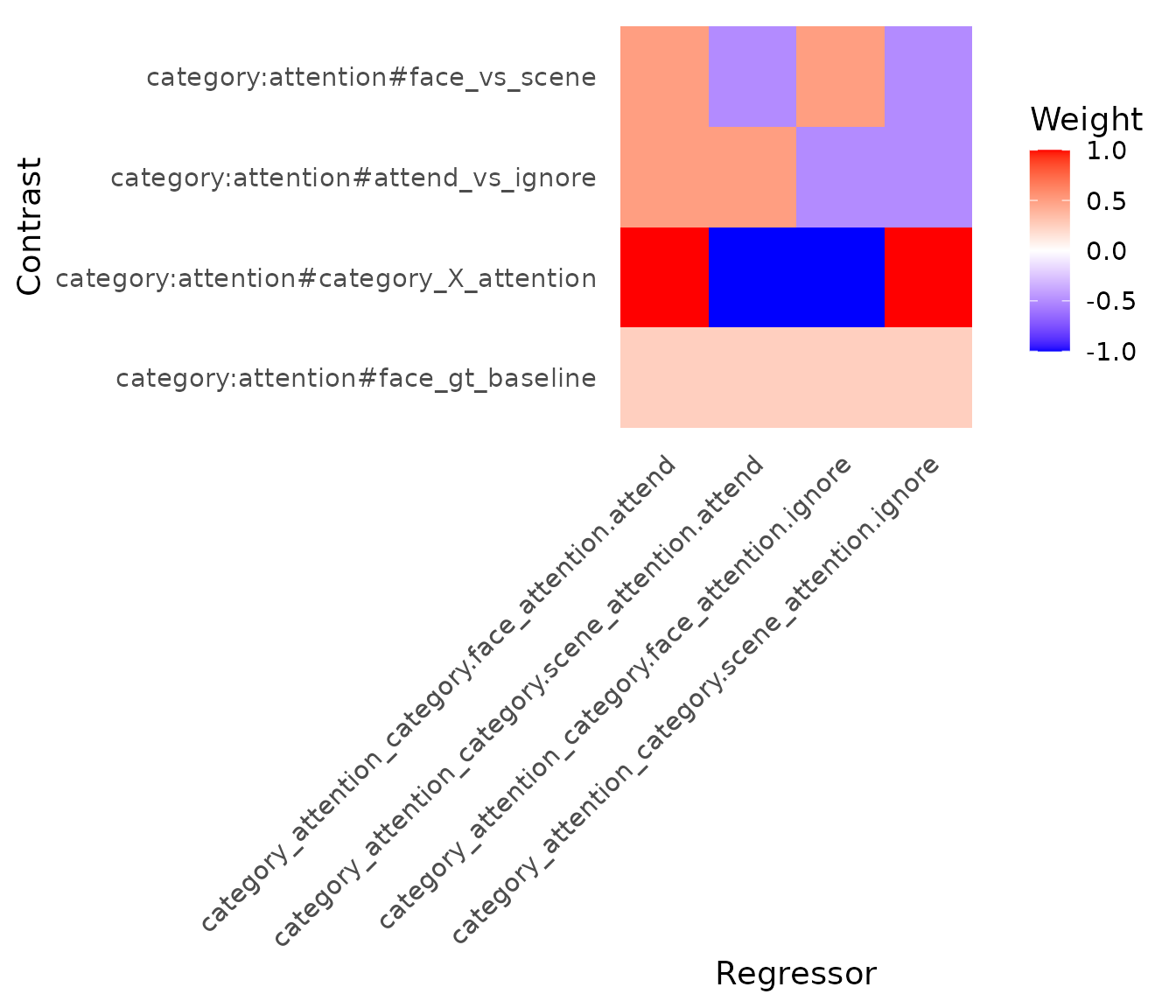 This plot helps verify that contrasts are specified correctly relative
to the full model design matrix.
This plot helps verify that contrasts are specified correctly relative
to the full model design matrix.
Working with Contrast Weights
The computed contrast weights can be used directly in statistical analyses or exported to other analysis packages. The weights matrix shows exactly how each experimental condition contributes to the contrast:
# View the structure of interaction contrast weights
cat("Interaction contrast structure:\n")
#> Interaction contrast structure:
str(wts_interaction)
#> List of 5
#>  $ term         :List of 9
#>   ..$ varname         : chr "category:attention"
#>   ..$ events          :List of 2
#>   .. ..$ category :List of 7
#>   .. .. ..$ varname   : chr "category"
#>   .. .. .. ..- attr(*, "orig_names")= chr "category"
#>   .. .. ..$ onsets    : num [1:8] 1 15.1 29.3 43.4 57.6 ...
#>   .. .. ..$ durations : num [1:8] 0 0 0 0 0 0 0 0
#>   .. .. ..$ blockids  : int [1:8] 1 1 1 1 1 1 1 1
#>   .. .. ..$ value     : int [1:8, 1] 1 2 1 2 1 2 1 2
#>   .. .. .. ..- attr(*, "dimnames")=List of 2
#>   .. .. .. .. ..$ : NULL
#>   .. .. .. .. ..$ : chr "category"
#>   .. .. .. .. .. ..- attr(*, "orig_names")= chr "category"
#>   .. .. ..$ continuous: logi FALSE
#>   .. .. ..$ meta      :List of 1
#>   .. .. .. ..$ levels: chr [1:2] "face" "scene"
#>   .. .. ..- attr(*, "class")= chr [1:2] "event" "event_seq"
#>   .. ..$ attention:List of 7
#>   .. .. ..$ varname   : chr "attention"
#>   .. .. .. ..- attr(*, "orig_names")= chr "attention"
#>   .. .. ..$ onsets    : num [1:8] 1 15.1 29.3 43.4 57.6 ...
#>   .. .. ..$ durations : num [1:8] 0 0 0 0 0 0 0 0
#>   .. .. ..$ blockids  : int [1:8] 1 1 1 1 1 1 1 1
#>   .. .. ..$ value     : int [1:8, 1] 1 1 2 2 1 1 2 2
#>   .. .. .. ..- attr(*, "dimnames")=List of 2
#>   .. .. .. .. ..$ : NULL
#>   .. .. .. .. ..$ : chr "attention"
#>   .. .. .. .. .. ..- attr(*, "orig_names")= chr "attention"
#>   .. .. ..$ continuous: logi FALSE
#>   .. .. ..$ meta      :List of 1
#>   .. .. .. ..$ levels: chr [1:2] "attend" "ignore"
#>   .. .. ..- attr(*, "class")= chr [1:2] "event" "event_seq"
#>   ..$ subset          : logi [1:8] TRUE TRUE TRUE TRUE TRUE TRUE ...
#>   ..$ event_table     : tibble [8 × 2] (S3: tbl_df/tbl/data.frame)
#>   .. ..$ category : Factor w/ 2 levels "face","scene": 1 2 1 2 1 2 1 2
#>   .. ..$ attention: Factor w/ 2 levels "attend","ignore": 1 1 2 2 1 1 2 2
#>   ..$ onsets          : num [1:8] 1 15.1 29.3 43.4 57.6 ...
#>   ..$ blockids        : int [1:8] 1 1 1 1 1 1 1 1
#>   ..$ durations       : num [1:8] 0 0 0 0 0 0 0 0
#>   ..$ condition_levels: chr [1:4] "category.face_attention.attend" "category.scene_attention.attend" "category.face_attention.ignore" "category.scene_attention.ignore"
#>   ..$ condition_ids   : int [1:8] 1 2 3 4 1 2 3 4
#>   ..- attr(*, "class")= chr [1:2] "event_term" "event_seq"
#>   ..- attr(*, "hrfspec")=List of 17
#>   .. ..$ name     : chr "category:attention"
#>   .. ..$ label    : chr "hrf(category,attention)"
#>   .. ..$ id       : NULL
#>   .. ..$ vars     :List of 2
#>   .. .. ..$ : language ~category
#>   .. .. .. ..- attr(*, ".Environment")=<environment: 0x55e103f1b420>
#>   .. .. ..$ : language ~attention
#>   .. .. .. ..- attr(*, ".Environment")=<environment: 0x55e103f1b420>
#>   .. .. ..- attr(*, "class")= chr [1:2] "quosures" "list"
#>   .. ..$ varnames : Named chr [1:2] "category" "attention"
#>   .. .. ..- attr(*, "names")= chr [1:2] "" ""
#>   .. ..$ hrf      :function (t)
#>   .. .. ..- attr(*, "class")= chr [1:2] "HRF" "function"
#>   .. .. ..- attr(*, "name")= chr "SPMG1"
#>   .. .. ..- attr(*, "nbasis")= int 1
#>   .. .. ..- attr(*, "span")= num 24
#>   .. .. ..- attr(*, "param_names")= chr [1:3] "P1" "P2" "A1"
#>   .. .. ..- attr(*, "params")=List of 3
#>   .. .. .. ..$ P1: num 5
#>   .. .. .. ..$ P2: num 15
#>   .. .. .. ..$ A1: num 0.0833
#>   .. ..$ hrf_fun  : NULL
#>   .. ..$ onsets   : NULL
#>   .. ..$ durations: NULL
#>   .. ..$ prefix   : NULL
#>   .. ..$ subset   : NULL
#>   .. ..$ precision: num 0.3
#>   .. ..$ contrasts: NULL
#>   .. ..$ summate  : logi TRUE
#>   .. ..$ normalize: logi FALSE
#>   .. ..$ uid      : chr "t01"
#>   .. ..$ term_tag : chr "category_attention"
#>   .. ..- attr(*, "class")= chr [1:2] "hrfspec" "list"
#>   ..- attr(*, "term_tag")= chr "category_attention"
#>   ..- attr(*, "uid")= chr "t01"
#>  $ name         : chr "category_X_attention"
#>  $ weights      : num [1:4, 1] 1 -1 -1 1
#>   ..- attr(*, "dimnames")=List of 2
#>   .. ..$ : chr [1:4] "category.face_attention.attend" "category.scene_attention.attend" "category.face_attention.ignore" "category.scene_attention.ignore"
#>   .. ..$ : NULL
#>  $ condnames    : chr [1:4] "category.face_attention.attend" "category.scene_attention.attend" "category.face_attention.ignore" "category.scene_attention.ignore"
#>  $ contrast_spec:List of 4
#>   ..$ A    :Class 'formula'  language ~(`face:attend` - `face:ignore`) - (`scene:attend` - `scene:ignore`)
#>   .. .. ..- attr(*, ".Environment")=<environment: R_GlobalEnv>
#>   ..$ B    : NULL
#>   ..$ where: NULL
#>   ..$ name : chr "category_X_attention"
#>   ..- attr(*, "class")= chr [1:3] "contrast_formula_spec" "contrast_spec" "list"
#>  - attr(*, "class")= chr [1:2] "contrast" "list"
cat("\nContrast weights matrix:\n")
#>
#> Contrast weights matrix:
print(wts_interaction$conmat)
#> NULL
Conclusion
The fmrireg package offers a comprehensive system for
defining and applying statistical contrasts in fMRI analysis. From
simple pairwise comparisons (pair_contrast) and baseline
tests (unit_contrast) to complex formula-based definitions
(contrast), trend analysis (poly_contrast),
and ANOVA-style effects (oneway_contrast,
interaction_contrast), researchers have fine-grained
control over hypothesis testing. The integration with
fmri_lm and visualization tools like
plot_contrasts facilitates robust and interpretable fMRI
modeling.
Next
-
vignette("benchmark_datasets", package = "fmrireg")— Benchmark datasets -
vignette("group_analysis", package = "fmrireg")— Group analysis