title: “06. Benchmark Datasets” author: “fmrireg package” date: “2025-09-01” output: rmarkdown::html_vignette vignette: > % % % —

Introduction

The fmrireg package includes a comprehensive set of benchmark datasets designed for testing and evaluating HRF fitting, beta estimation, and other fMRI analysis methods. These datasets provide known ground truth for various challenging scenarios commonly encountered in fMRI analysis.

This vignette demonstrates how to use these benchmark datasets to evaluate your analysis methods.

library(fmrireg)
#> 
#> Attaching package: 'fmrireg'
#> The following object is masked from 'package:stats':
#> 
#>     convolve
library(ggplot2)
library(dplyr)
#> 
#> Attaching package: 'dplyr'
#> The following object is masked from 'package:fmrireg':
#> 
#>     group_data
#> The following objects are masked from 'package:stats':
#> 
#>     filter, lag
#> The following objects are masked from 'package:base':
#> 
#>     intersect, setdiff, setequal, union

Available Benchmark Datasets

Let’s start by exploring what benchmark datasets are available:

# List all available datasets
datasets_info <- list_benchmark_datasets()
print(datasets_info)
#>                                                         Dataset
#> BM_Canonical_HighSNR                       BM_Canonical_HighSNR
#> BM_Canonical_LowSNR                         BM_Canonical_LowSNR
#> BM_HRF_Variability_AcrossVoxels BM_HRF_Variability_AcrossVoxels
#> BM_Trial_Amplitude_Variability   BM_Trial_Amplitude_Variability
#> BM_Complex_Realistic                       BM_Complex_Realistic
#>                                                                                                                        Description
#> BM_Canonical_HighSNR                                 Canonical HRF (SPMG1), high SNR, 3 conditions, fixed amplitudes per condition
#> BM_Canonical_LowSNR                                   Canonical HRF (SPMG1), low SNR, 3 conditions, fixed amplitudes per condition
#> BM_HRF_Variability_AcrossVoxels                                         HRF varies across voxel groups, 2 conditions, moderate SNR
#> BM_Trial_Amplitude_Variability                              Single condition with significant trial-to-trial amplitude variability
#> BM_Complex_Realistic            Complex realistic scenario: 3 HRF groups, 3 conditions, variable durations/amplitudes, AR(2) noise

Loading and Exploring a Dataset

Let’s load the high SNR canonical dataset and explore its structure:

# Load the high SNR dataset
data <- load_benchmark_dataset("BM_Canonical_HighSNR")

# Get a summary of the dataset
summary_info <- get_benchmark_summary("BM_Canonical_HighSNR")
print(summary_info$dimensions)
#> $n_timepoints
#> [1] 150
#> 
#> $n_voxels
#> [1] 100
#> 
#> $n_events
#> [1] 45
#> 
#> $n_conditions
#> [1] 3
print(summary_info$experimental_design)
#> $conditions
#> [1] "Cond1" "Cond2" "Cond3"
#> 
#> $events_per_condition
#> $events_per_condition$Cond1
#> [1] 15
#> 
#> $events_per_condition$Cond2
#> [1] 15
#> 
#> $events_per_condition$Cond3
#> [1] 15
#> 
#> 
#> $TR
#> [1] 2
#> 
#> $total_time
#> [1] 300
#> 
#> $target_snr
#> [1] 4

Next

• 07 Group Analysis

Examining the Data Structure

Each benchmark dataset is a list. Key components include:

• description: A text summary.
• Y_noisy: The matrix of noisy BOLD time series (time points x voxels).
• Y_clean: (When available) The BOLD signal without noise.
• event_onsets: Vector of event start times.
• condition_labels: Vector of condition names for each event.
• event_durations: Vector of event durations.
• true_betas_condition: Ground truth beta values for each condition.
• true_hrf_parameters: Information about the HRF used in simulation.
• TR, total_time, run_length: Scan parameters.

# Look at the BOLD time series dimensions and event structure
cat("Y_noisy BOLD data dimensions:", dim(data$Y_noisy), "\n")
#> Y_noisy BOLD data dimensions: 150 100
cat("Number of events:", length(data$event_onsets), "\n")
#> Number of events: 45
cat("Conditions:", unique(data$condition_labels), "\n")
#> Conditions: Cond1 Cond2 Cond3
cat("Events per condition:", table(data$condition_labels), "\n")
#> Events per condition: 15 15 15
cat("TR:", data$TR, "\n")
#> TR: 2
cat("Run length:", data$run_length, "\n")
#> Run length:

Visualizing the Data

Let’s visualize some aspects of the benchmark dataset:

# Plot the first few voxels' time series
n_timepoints <- nrow(data$Y_noisy)
time_points <- seq(0, by = data$TR, length.out = n_timepoints)

# Create a data frame for plotting
plot_data <- data.frame(
  Time = rep(time_points, 3),
  BOLD = c(data$Y_noisy[, 1], data$Y_noisy[, 2], data$Y_noisy[, 3]),
  Voxel = rep(paste("Voxel", 1:3), each = n_timepoints)
)

# Add event markers
event_data <- data.frame(
  Time = data$event_onsets,
  Condition = data$condition_labels
)

ggplot(plot_data, aes(x = Time, y = BOLD)) +
  geom_line() +
  geom_vline(data = event_data, aes(xintercept = Time, color = Condition), 
             alpha = 0.7, linetype = "dashed") +
  facet_wrap(~Voxel, scales = "free_y") +
  labs(title = "BOLD Time Series with Event Markers",
       x = "Time (seconds)", y = "BOLD Signal") +
  theme_minimal()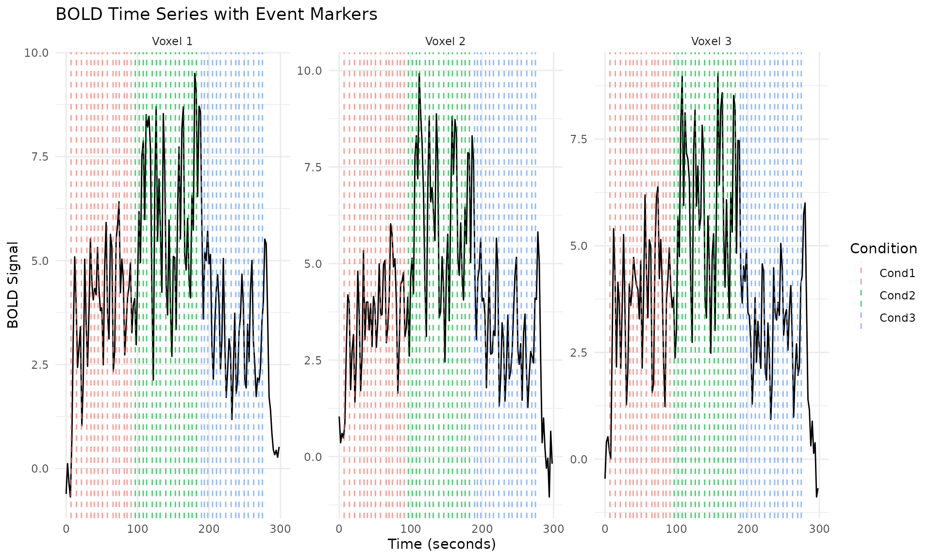

Creating Design Matrices

One of the key features is the ability to create design matrices with different HRF assumptions:

# Create design matrix with the true HRF (canonical)
X_true <- create_design_matrix_from_benchmark("BM_Canonical_HighSNR", fmrihrf::HRF_SPMG1)

# Create design matrix with a different HRF (e.g., a Gaussian HRF instead of canonical)
X_wrong <- create_design_matrix_from_benchmark("BM_Canonical_HighSNR", fmrihrf::HRF_GAUSSIAN)

cat("True HRF design matrix dimensions:", dim(X_true), "\n")
#> True HRF design matrix dimensions: 150 4
cat("Alternative HRF design matrix dimensions:", dim(X_wrong), "\n")
#> Alternative HRF design matrix dimensions: 150 4

Method Evaluation Example

Let’s demonstrate how to evaluate a simple method (OLS) on the benchmark dataset:

# Fit ordinary least squares with the correct HRF
betas_correct <- solve(t(X_true) %*% X_true) %*% t(X_true) %*% data$Y_noisy

# Fit OLS with the wrong HRF assumption
betas_wrong <- solve(t(X_wrong) %*% X_wrong) %*% t(X_wrong) %*% data$Y_noisy

# Evaluate performance (remove intercept for comparison)
performance_correct <- evaluate_method_performance("BM_Canonical_HighSNR", 
                                                   betas_correct[-1, ], 
                                                   "OLS_Correct_HRF")

performance_wrong <- evaluate_method_performance("BM_Canonical_HighSNR", 
                                                 betas_wrong[-1, ], 
                                                 "OLS_Wrong_HRF")

# Compare results
cat("Correct HRF - Overall correlation:", round(performance_correct$overall_metrics$correlation, 3), "\n")
#> Correct HRF - Overall correlation: 0.989
cat("Wrong HRF - Overall correlation:", round(performance_wrong$overall_metrics$correlation, 3), "\n")
#> Wrong HRF - Overall correlation: 0.99

cat("Correct HRF - RMSE:", round(performance_correct$overall_metrics$rmse, 3), "\n")
#> Correct HRF - RMSE: 0.044
cat("Wrong HRF - RMSE:", round(performance_wrong$overall_metrics$rmse, 3), "\n")
#> Wrong HRF - RMSE: 8.415

Comparing True vs Estimated Betas

# Get true betas
true_betas <- data$true_betas_condition

# Create comparison plots
comparison_data <- data.frame(
  True = as.vector(true_betas),
  Estimated_Correct = as.vector(betas_correct[-1, ]),
  Estimated_Wrong = as.vector(betas_wrong[-1, ]),
  Condition = rep(paste("Condition", 1:3), each = ncol(true_betas))
)

# Plot true vs estimated (correct HRF)
p1 <- ggplot(comparison_data, aes(x = True, y = Estimated_Correct, color = Condition)) +
  geom_point(alpha = 0.6) +
  geom_abline(slope = 1, intercept = 0, linetype = "dashed") +
  labs(title = "Correct HRF", x = "True Beta", y = "Estimated Beta") +
  theme_minimal()

# Plot true vs estimated (wrong HRF)
p2 <- ggplot(comparison_data, aes(x = True, y = Estimated_Wrong, color = Condition)) +
  geom_point(alpha = 0.6) +
  geom_abline(slope = 1, intercept = 0, linetype = "dashed") +
  labs(title = "Wrong HRF", x = "True Beta", y = "Estimated Beta") +
  theme_minimal()

# Display plots side by side
gridExtra::grid.arrange(p1, p2, ncol = 2)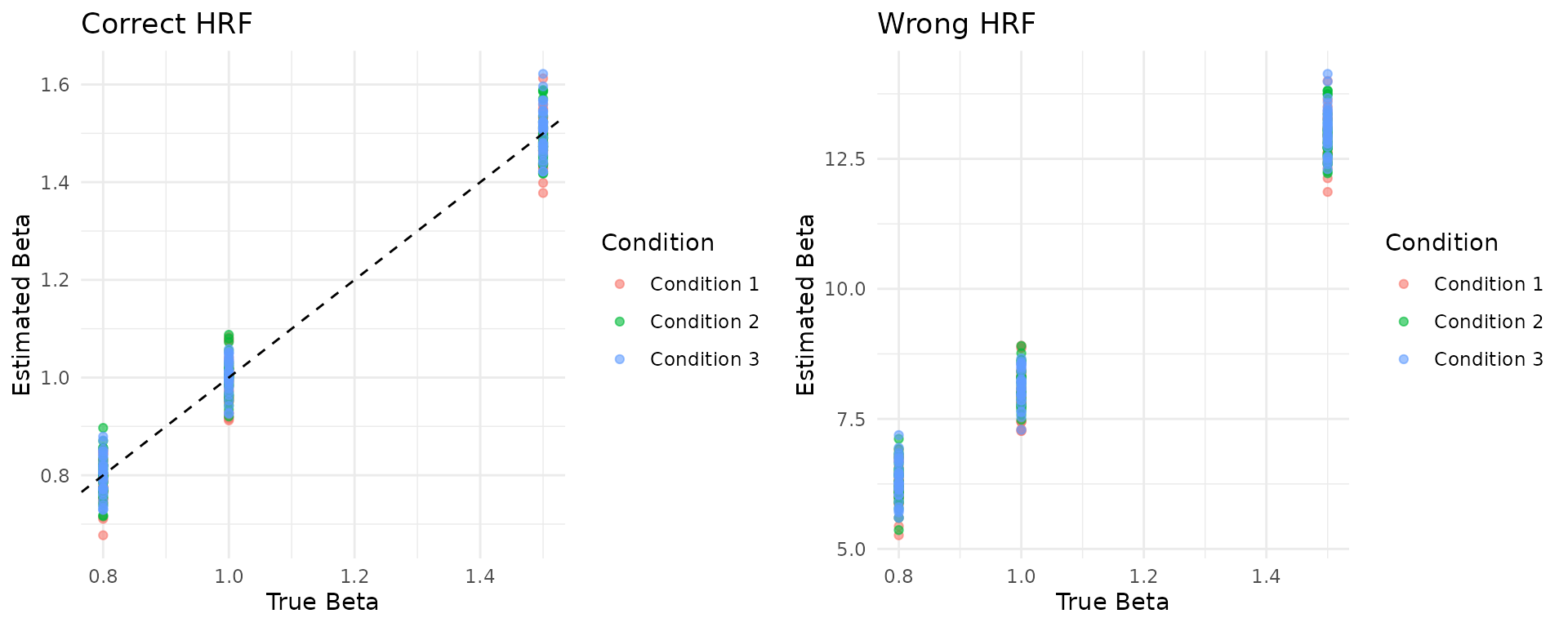

Testing Different Datasets

Let’s compare performance across different benchmark scenarios:

# Test on different datasets
datasets_to_test <- c("BM_Canonical_HighSNR", "BM_Canonical_LowSNR")
results <- list()

for (dataset_name in datasets_to_test) {
  # Load dataset and create design matrix
  X <- create_design_matrix_from_benchmark(dataset_name, fmrihrf::HRF_SPMG1)
  data_test <- load_benchmark_dataset(dataset_name)
  
  # Fit model
  betas <- solve(t(X) %*% X) %*% t(X) %*% data_test$Y_noisy
  
  # Evaluate performance
  perf <- evaluate_method_performance(dataset_name, betas[-1, ], "OLS")
  
  results[[dataset_name]] <- list(
    correlation = perf$overall_metrics$correlation,
    rmse = perf$overall_metrics$rmse,
    target_snr = data_test$target_snr
  )
}

# Display results
results_df <- data.frame(
  Dataset = names(results),
  Correlation = sapply(results, function(x) round(x$correlation, 3)),
  RMSE = sapply(results, function(x) round(x$rmse, 3)),
  Target_SNR = sapply(results, function(x) x$target_snr)
)

print(results_df)
#>                                   Dataset Correlation  RMSE Target_SNR
#> BM_Canonical_HighSNR BM_Canonical_HighSNR       0.989 0.044        4.0
#> BM_Canonical_LowSNR   BM_Canonical_LowSNR       0.595 0.410        0.5

HRF Variability Dataset

Let’s explore the dataset with HRF variability across voxels:

# Load the HRF variability dataset
hrf_data <- load_benchmark_dataset("BM_HRF_Variability_AcrossVoxels")

# Examine the HRF group assignments
cat("HRF group assignments:", table(hrf_data$true_hrf_group_assignment), "\n")
#> HRF group assignments: 50 50

# Note: The actual HRF objects used vary by voxel
# The benchmark dataset contains voxels with different HRF shapes to test
# methods that can handle HRF variability across the brain

Trial Amplitude Variability

Let’s examine the trial-to-trial variability dataset:

# Load the trial variability dataset
trial_data <- load_benchmark_dataset("BM_Trial_Amplitude_Variability")

# Look at the trial-wise amplitudes
true_trial_amps <- trial_data$true_amplitudes_trial

# Plot amplitude variability across trials for first few voxels
amp_plot_data <- data.frame(
  Trial = rep(1:nrow(true_trial_amps), 3),
  Amplitude = c(true_trial_amps[, 1], true_trial_amps[, 2], true_trial_amps[, 3]),
  Voxel = rep(paste("Voxel", 1:3), each = nrow(true_trial_amps))
)

ggplot(amp_plot_data, aes(x = Trial, y = Amplitude)) +
  geom_line() +
  geom_point() +
  facet_wrap(~Voxel) +
  labs(title = "Trial-to-Trial Amplitude Variability",
       x = "Trial Number", y = "True Amplitude") +
  theme_minimal()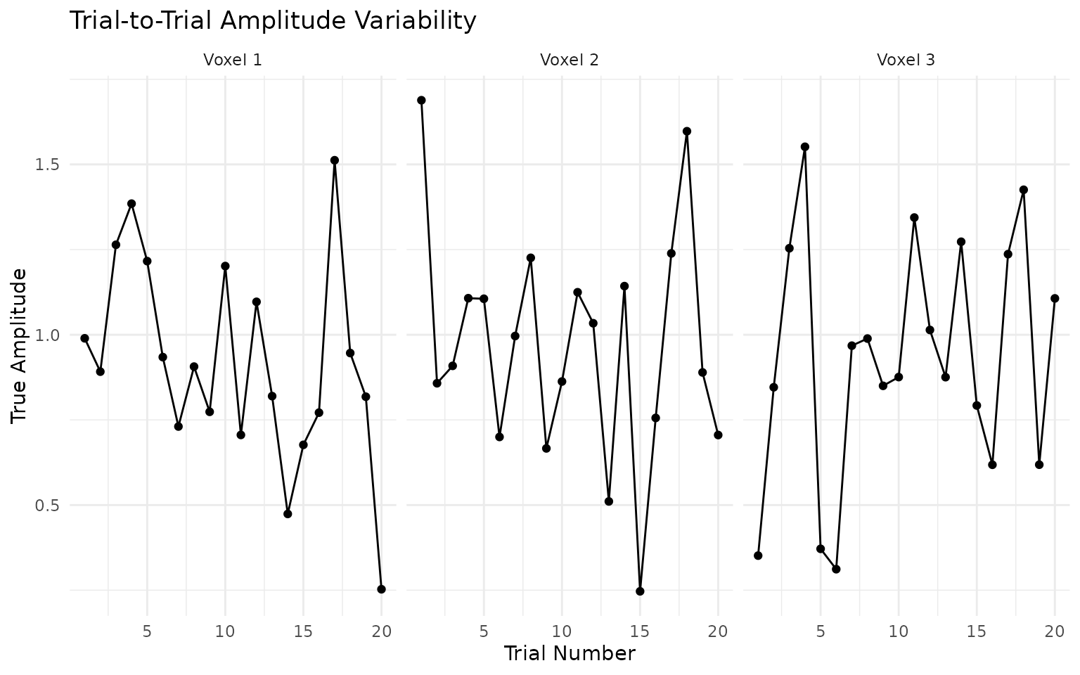

Summary

The fMRI benchmark datasets provide a comprehensive testing framework for:

1. Basic validation: Use BM_Canonical_HighSNR for initial method testing
2. Noise robustness: Compare performance between high and low SNR datasets
3. HRF estimation: Test methods on BM_HRF_Variability_AcrossVoxels
4. Single-trial analysis: Evaluate LSS methods on BM_Trial_Amplitude_Variability
5. Complex scenarios: Challenge methods with BM_Complex_Realistic

Key advantages:

• Known ground truth: All parameters are precisely controlled and recorded
• Realistic noise models: AR(1) and AR(2) noise with physiologically plausible parameters
• Comprehensive evaluation: Built-in performance metrics and comparison tools
• Reproducible: Fixed random seeds ensure consistent results
• Extensible: Framework allows easy addition of new benchmark scenarios

These datasets enable rigorous, standardized evaluation of fMRI analysis methods and facilitate fair comparisons between different approaches.