The OASIS Method: Optimized Analytic Single-pass Inverse Solution • fmrilss

library(fmrihrf)
library(fmrilss)
set.seed(42)

What OASIS Adds Over Plain LSS

When you call lss() with a single-basis HRF and no ridge penalty, the optimized backends already factor the shared structure across trials into a single-pass solve. OASIS wraps that same estimator in a richer workflow.

You get automatic design construction from event onsets via fmrihrf, multi-basis HRF support (K > 1), ridge regularization, analytical standard errors, and optional AR(1) prewhitening—all in one call. If you only need the leanest single-basis path, stick with method = "cpp_optimized".

Synthetic Data

We generate a rapid event-related dataset with jittered ISIs and known ground-truth betas.

n_time   <- 300
n_voxels <- 100
TR       <- 1.0
sframe   <- fmrihrf::sampling_frame(blocklens = n_time, TR = TR)

isi    <- runif(500, min = 3, max = 9)
onsets <- cumsum(c(10, isi))
onsets <- onsets[onsets < (n_time - 20)]
n_trials <- length(onsets)

true_betas <- matrix(rnorm(n_trials * n_voxels, mean = 1, sd = 0.5),
                     n_trials, n_voxels)
grid <- fmrihrf::samples(sframe, global = TRUE)
rset <- fmrihrf::regressor_set(
  onsets = onsets, fac = factor(seq_len(n_trials)),
  hrf = fmrihrf::HRF_SPMG1, duration = 0, span = 30, summate = FALSE
)
X_trials <- fmrihrf::evaluate(rset, grid = grid, precision = 0.1, method = "conv")

Y <- matrix(rnorm(n_time * n_voxels), n_time, n_voxels)
Y <- Y + X_trials %*% true_betas

Basic OASIS Call

Pass a design_spec instead of a pre-built X and let OASIS construct the trial-wise design internally.

beta_oasis <- lss(
  Y = Y, X = NULL, method = "oasis",
  oasis = list(design_spec = list(
    sframe = sframe,
    cond   = list(onsets = onsets, hrf = fmrihrf::HRF_SPMG1, span = 30)
  ))
)
dim(beta_oasis)
#> [1]  42 100

The result is an n_trials x n_voxels matrix, exactly the same shape you get from the other LSS backends. By default, OASIS applies 5% fractional ridge regularization, which is worth keeping in mind when you compare it to unregularized LSS fits.

Equivalence to LSS

With a single-basis HRF and no ridge penalty, OASIS returns the same coefficients as the optimized LSS path. You can verify this up to floating-point tolerance.

Z <- cbind(1, scale(1:n_time))
b_lss   <- lss(Y, X_trials, Z = Z, method = "cpp_optimized")
b_oasis <- lss(Y, X_trials, Z = Z, method = "oasis",
               oasis = list(ridge_mode = "absolute", ridge_x = 0, ridge_b = 0))
equiv_err <- max(abs(b_lss - b_oasis))
equiv_err

Use the plain LSS backends when you have a fixed single-basis X and want the leanest dependency surface. Prefer OASIS when you need built-in design construction, multi-basis HRFs, ridge, or standard errors.

Ridge Regularization

In rapid designs, close trial spacing produces correlated regressors. Ridge regression trades a small bias for a large variance reduction. OASIS offers two modes.

Absolute Ridge

You specify fixed penalty values added to the diagonal of the per-trial normal equations.

beta_noridge <- lss(
  Y = Y, X = NULL, method = "oasis",
  oasis = list(
    design_spec = list(sframe = sframe,
      cond = list(onsets = onsets, hrf = fmrihrf::HRF_SPMG1, span = 30)),
    ridge_mode = "absolute", ridge_x = 0, ridge_b = 0
  )
)

beta_abs <- lss(
  Y = Y, X = NULL, method = "oasis",
  oasis = list(
    design_spec = list(sframe = sframe,
      cond = list(onsets = onsets, hrf = fmrihrf::HRF_SPMG1, span = 30)),
    ridge_mode = "absolute", ridge_x = 0.1, ridge_b = 0.1
  )
)

Fractional Ridge

The penalty scales relative to the mean diagonal energy in the design, adapting automatically to your data. A 5% fractional ridge is also the package default when you do not override the ridge settings.

beta_frac <- lss(
  Y = Y, X = NULL, method = "oasis",
  oasis = list(
    design_spec = list(sframe = sframe,
      cond = list(onsets = onsets, hrf = fmrihrf::HRF_SPMG1, span = 30)),
    ridge_mode = "fractional", ridge_x = 0.05, ridge_b = 0.05
  )
)

Notice the variance reduction compared to the unregularized estimates:

ridge_summary <- data.frame(
  Fit = c("No ridge", "Fractional 5%"),
  MeanTrialVariance = c(
    mean(apply(beta_noridge, 2, var)),
    mean(apply(beta_frac, 2, var))
  )
)
ridge_summary
#>             Fit MeanTrialVariance
#> 1      No ridge         0.3679561
#> 2 Fractional 5%         0.3330022

Practical starting points for fractional ridge: 0.005 for well-separated trials (ISI >= 6 s), 0.01 for typical rapid designs, and 0.02–0.05 for very dense events or multi-basis models. See ?lss for details.

Multi-Basis HRFs

Multi-basis models capture trial-to-trial variability in HRF shape. OASIS returns K rows per trial, interleaved by basis.

beta_spmg3 <- lss(
  Y = Y, X = NULL, method = "oasis",
  oasis = list(design_spec = list(
    sframe = sframe,
    cond = list(onsets = onsets, hrf = fmrihrf::HRF_SPMG3, span = 30)
  ))
)
dim(beta_spmg3)
#> [1] 126 100

With K = 3 (canonical + temporal derivative + dispersion derivative), the output has K * n_trials rows. Extract each component using the K-stride pattern.

K <- 3
canonical  <- beta_spmg3[seq(1, nrow(beta_spmg3), by = K), ]
temporal   <- beta_spmg3[seq(2, nrow(beta_spmg3), by = K), ]
dispersion <- beta_spmg3[seq(3, nrow(beta_spmg3), by = K), ]
cat("Each component:", nrow(canonical), "trials x", ncol(canonical), "voxels\n")
#> Each component: 42 trials x 100 voxels

Large temporal-derivative weights suggest timing variability across trials; dispersion-derivative weights indicate width changes.

FIR Basis

The Finite Impulse Response basis makes no parametric assumptions about HRF shape. Each trial contributes one coefficient per time bin.

fir_hrf  <- fmrihrf::hrf_fir_generator(nbasis = 15, span = 30)
beta_fir <- lss(
  Y = Y, X = NULL, method = "oasis",
  oasis = list(
    design_spec = list(sframe = sframe,
      cond = list(onsets = onsets, hrf = fir_hrf, span = 30)),
    ridge_mode = "fractional", ridge_x = 0.2, ridge_b = 0.2
  )
)
dim(beta_fir)
#> [1] 630 100

Moderate ridge is important here because FIR fits are high-dimensional. You can average across trials and voxels to recover a smooth HRF estimate.

n_bins    <- 15
bin_width <- 30 / n_bins
fir_array <- array(beta_fir, dim = c(n_bins, n_trials, n_voxels))
fir_mean  <- apply(fir_array, 1, mean)
fir_se    <- apply(fir_array, 1, sd) / sqrt(n_trials * n_voxels)
tp        <- seq(0, (n_bins - 1) * bin_width, by = bin_width)

plot(tp, fir_mean, type = "l", col = "navy", lwd = 2,
     main = "FIR-derived HRF", xlab = "Time (s)", ylab = "Response")
polygon(c(tp, rev(tp)), c(fir_mean + fir_se, rev(fir_mean - fir_se)),
        col = grDevices::adjustcolor("navy", 0.2), border = NA)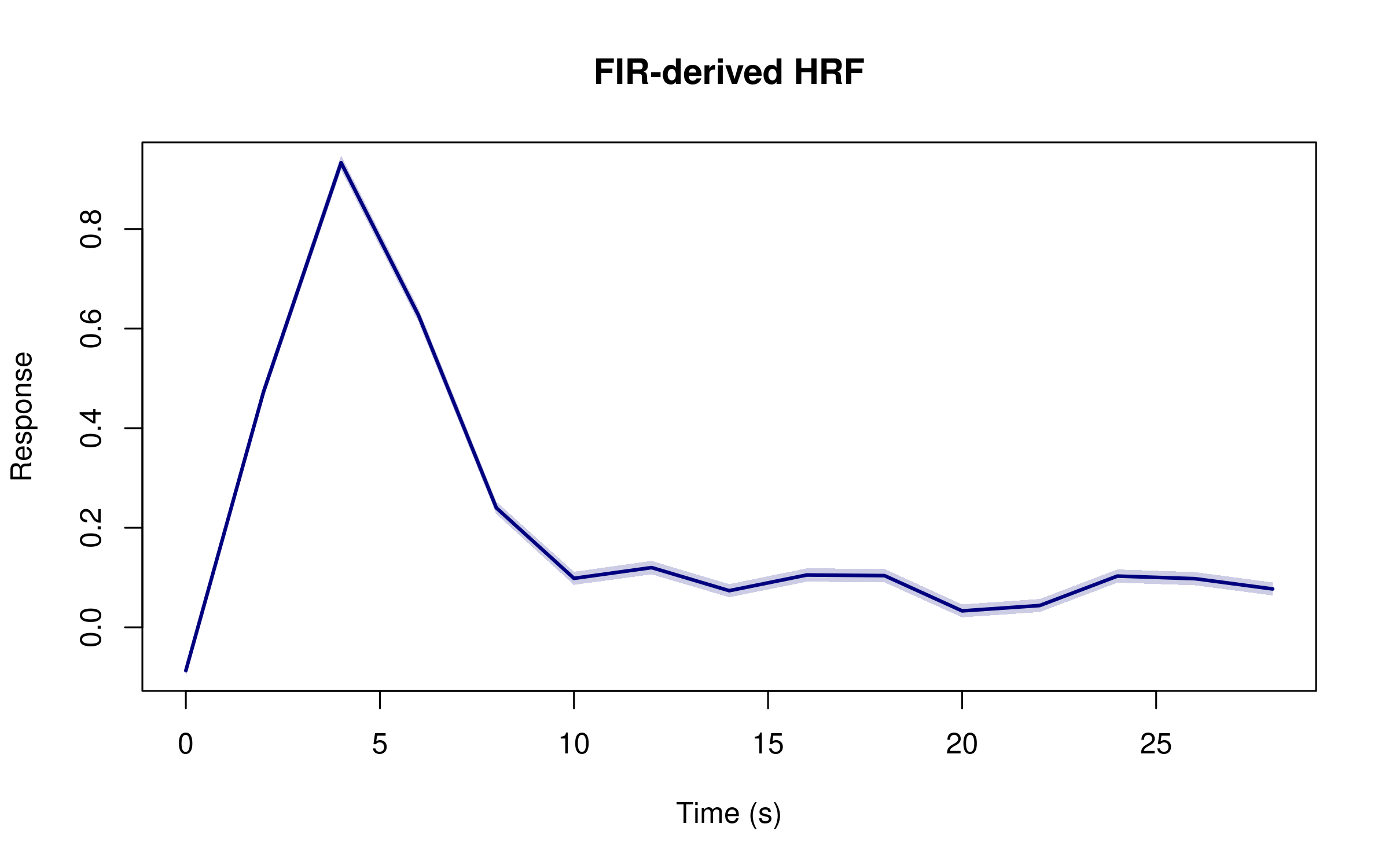

FIR-derived mean HRF with SE ribbon.

HRF Grid Search

When you are unsure which HRF shape fits best, pass a candidate grid via hrf_grid and let OASIS pick a single global winner using a matched-filter score.

hrf_grid <- create_lwu_grid(
  tau_range = c(4, 8), sigma_range = c(2, 3.5),
  rho_range = c(0.2, 0.5), n_tau = 3, n_sigma = 2, n_rho = 2
)

beta_grid <- lss(
  Y = Y, X = NULL, method = "oasis",
  oasis = list(
    design_spec = list(sframe = sframe,
      cond = list(onsets = onsets, span = 30),
      hrf_grid = hrf_grid$hrfs),
    ridge_mode = "fractional", ridge_x = 0.01, ridge_b = 0.01
  )
)
dim(beta_grid)

This selects a single HRF shared across all voxels, then refits with it. For voxel-specific HRF estimation, see vignette("voxel-wise-hrf").

Multiple Conditions

Real experiments often have multiple conditions. Place your target condition in cond and other conditions in others so their variance is accounted for as nuisance.

onsets_a <- seq(10, 280, by = 30)
onsets_b <- seq(25, 280, by = 30)

beta_multi <- lss(
  Y = Y, X = NULL, method = "oasis",
  oasis = list(design_spec = list(
    sframe = sframe,
    cond   = list(onsets = onsets_a, hrf = fmrihrf::HRF_SPMG1, span = 30),
    others = list(list(onsets = onsets_b))
  ))
)
dim(beta_multi)
#> [1]  10 100

The others list ensures that condition B’s variance is accounted for when estimating condition A betas, preventing omitted-variable bias.

Standard Errors

Request analytical standard errors with return_se = TRUE. You can then compute trial-level t-statistics directly.

res_se <- lss(
  Y = Y[, 1:10], X = NULL, method = "oasis",
  oasis = list(
    design_spec = list(sframe = sframe,
      cond = list(onsets = onsets, hrf = fmrihrf::HRF_SPMG1, span = 30)),
    return_se = TRUE
  )
)

t_stats <- res_se$beta / res_se$se
cat("Mean |t|:", round(mean(abs(t_stats)), 2), "\n")
#> Mean |t|: 2.77

Trials with larger standard errors typically have more overlapping neighbours or occur during noisier periods.

Prewhitening

fMRI time series are temporally autocorrelated. You can apply AR(1) prewhitening so that standard errors and t-statistics are valid.

beta_pw <- lss(
  Y = Y[, 1:10], X = NULL, method = "oasis",
  oasis = list(design_spec = list(sframe = sframe,
    cond = list(onsets = onsets, hrf = fmrihrf::HRF_SPMG1, span = 30))),
  prewhiten = list(method = "ar", p = 1)
)
dim(beta_pw)
#> [1] 42 10

OASIS applies the whitening transform consistently to data, trial design, and nuisance regressors. For advanced options (auto AR order selection, voxel-wise or parcel-based pooling, ARMA models), see ?lss.

When to Use OASIS

Prefer OASIS when you want HRF-aware design construction, multi-basis HRFs (K > 1), ridge regularization, or standard errors in one call. It is especially useful for rapid event-related designs with hundreds of trials.

Prefer standard LSS backends when you already have a single-basis design matrix X and want the leanest, most transparent code path.

Next Steps

vignette("fmrilss") — foundational LSS concepts
vignette("voxel-wise-hrf") — spatial HRF modeling
vignette("sbhm") — library-constrained voxel-specific HRFs
vignette("oasis_theory") — mathematical details