Shared-Basis HRF Matching (SBHM): Efficient Voxel-Specific HRF Estimation

The Problem

Real fMRI data shows substantial HRF variability across brain regions. A single canonical HRF often fits poorly, but estimating fully unconstrained voxel-wise HRFs is expensive and noisy. SBHM offers a middle path: learn a shared basis from a library of plausible HRFs, then match each voxel to its best library member in a low-dimensional space.

The pipeline has four steps:

1. Build a shared basis from an HRF library via SVD (sbhm_build())
2. Prepass aggregate model fit per voxel (sbhm_prepass())
3. Match voxels to library members by cosine similarity (sbhm_match())
4. Project trial-wise coefficients to scalar amplitudes (sbhm_project())

In practice, lss_sbhm() runs all four steps in a single call.

library(fmrihrf)
library(fmrilss)

# Derived convenience defaults for examples
n_voxels_default <- if (fast_mode) 20 else 50
n_trials_default <- if (fast_mode) 6 else 10
ranks_default    <- if (fast_mode) 2:6 else 2:10

Step 1: Build the Shared Basis

We start by defining a grid of gamma HRF parameters spanning physiological variability in peak time and width.

shapes <- if (fast_mode) seq(6, 10, by = 2) else seq(5, 11, by = 1.5)
rates  <- if (fast_mode) seq(0.8, 1.2, by = 0.2) else seq(0.7, 1.3, by = 0.15)
param_grid <- expand.grid(shape = shapes, rate = rates)
cat("Library size:", nrow(param_grid), "HRFs\n")
#> Library size: 9 HRFs

Each grid row becomes a gamma HRF. We wrap this in a factory function that sbhm_build() can evaluate across the grid.

gamma_fun <- function(shape, rate) {
  f <- function(t) fmrihrf::hrf_gamma(t, shape = shape, rate = rate)
  fmrihrf::as_hrf(f, name = sprintf("gamma(s=%.2f,r=%.2f)", shape, rate), span = 32)
}

Now we build the SBHM basis. The SVD decomposes the library into a shared time basis B, singular values S, and per-HRF coordinates A.

sframe <- sampling_frame(blocklens = n_time, TR = TR)
sbhm <- sbhm_build(
  library_spec = list(fun = gamma_fun, pgrid = param_grid, span = 32,
                      precision = 0.1, method = "conv"),
  r = 6, sframe = sframe,
  baseline = c(0, 0.5), normalize = TRUE, ref = "mean"
)

cat("B (time basis):", dim(sbhm$B), "\n")
#> B (time basis): 160 6
cat("A (library coords):", dim(sbhm$A), "\n")
#> A (library coords): 6 9
cat("Singular values:", round(sbhm$S, 2), "\n")
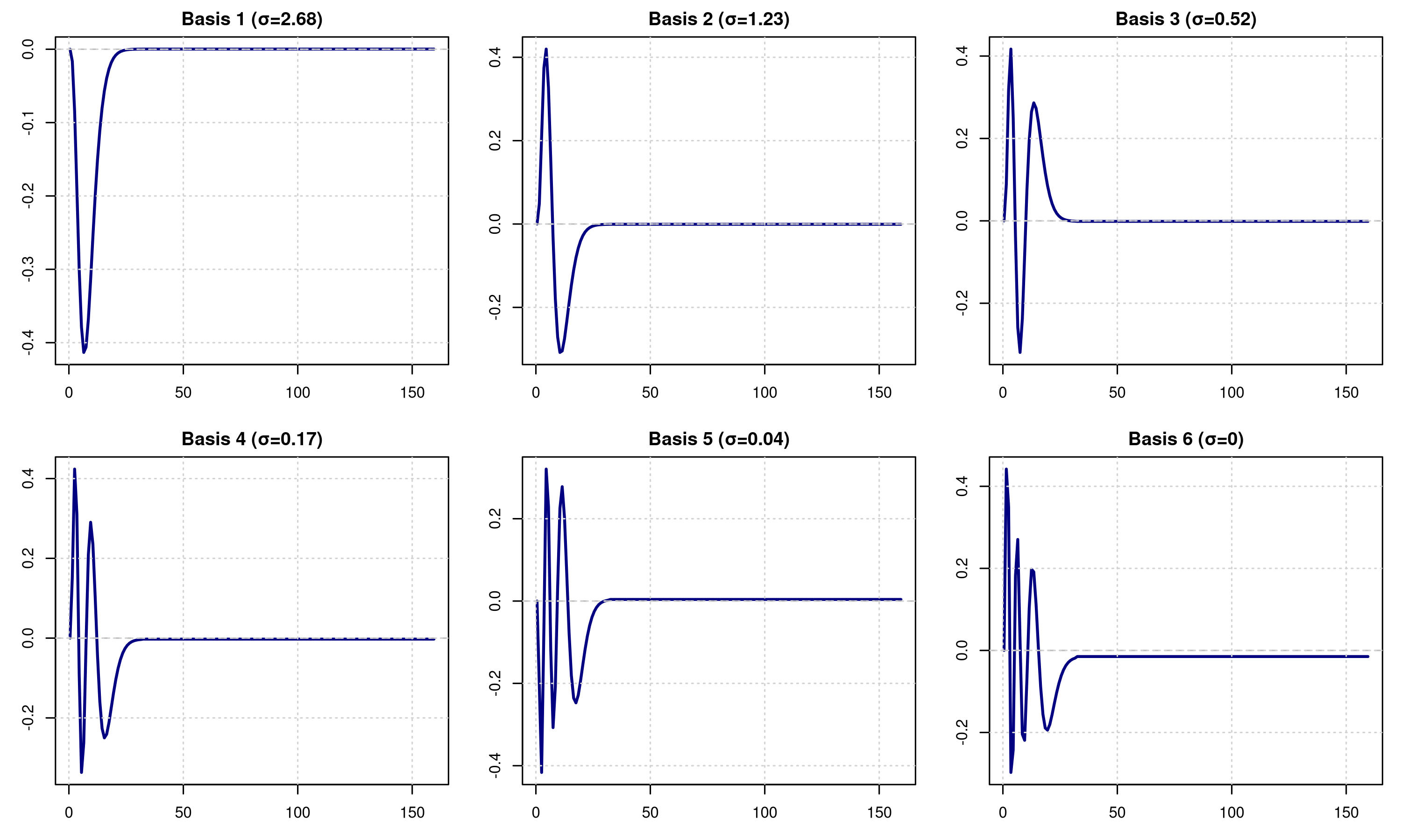
#> Singular values: 2.68 1.23 0.52 0.17 0.04 0

Visualizing the Basis

Each basis function captures a principal mode of HRF variation: the main shape, timing shifts, width differences, and undershoot features.

par(mfrow = c(2, 3), mar = c(3, 3, 2, 1))
for (i in 1:ncol(sbhm$B)) {
  plot(sbhm$tgrid, sbhm$B[, i], type = "l", col = "navy", lwd = 2,
       main = paste0("Basis ", i, " (s=", round(sbhm$S[i], 2), ")"),
       xlab = "Time (s)", ylab = "Amplitude")
  abline(h = 0, col = "gray", lty = 2)
}

Choosing the Rank

Aim for 90–95% variance explained. We can sweep ranks to find the elbow.

ranks <- ranks_default
ve <- sapply(ranks, function(ri) {
  sum(sbhm_build(library_spec = list(fun = gamma_fun, pgrid = param_grid, span = 32),
                 r = ri, sframe = sframe, normalize = TRUE)$S^2)
})

plot(ranks, ve / max(ve) * 100, type = "b", pch = 19, col = "navy",
     lwd = 2, xlab = "Rank (r)", ylab = "Variance Explained (%)",
     main = "Choosing SBHM Rank")
abline(h = 95, col = "red", lty = 2)
grid()

Library Coverage

A sample of rank-r reconstructed HRFs shows the range of shapes the library spans.

H_hat <- sbhm$B %*% sbhm$A
sel <- unique(round(seq(1, ncol(H_hat), length.out = min(ncol(H_hat), 12))))
matplot(sbhm$tgrid, H_hat[, sel, drop = FALSE], type = "l", lty = 1,
        col = colorRampPalette(c("#6baed6", "#08519c"))(length(sel)),
        lwd = 1.5, xlab = "Time (s)", ylab = "Amplitude",
        main = "Sample of Library HRFs (rank-r reconstruction)")
abline(h = 0, col = "gray80", lty = 2)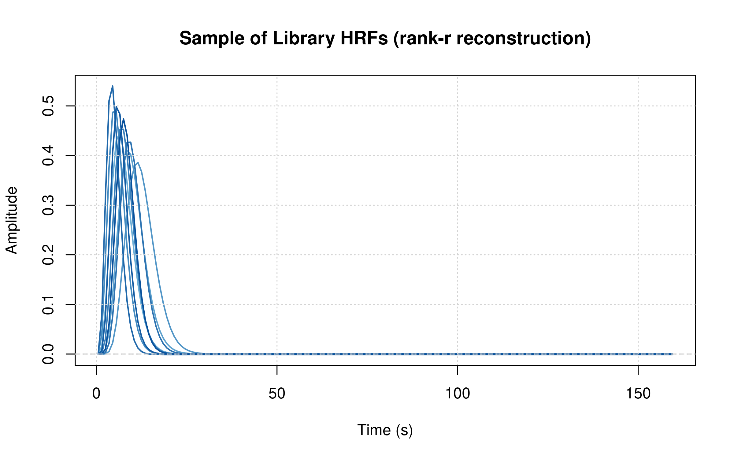

Step 2: Generate Synthetic Data

To demonstrate recovery, we create data where each voxel uses a known HRF from the library. First, set up the experimental design.

n_voxels <- n_voxels_default
n_trials <- n_trials_default
safe_end <- max(sbhm$tgrid) - 30
onsets <- seq(20, safe_end, length.out = n_trials)

Assign each voxel a random library HRF and build per-trial regressors. The fresh set.seed() here keeps the HRF assignment reproducible independently of earlier random draws.

set.seed(456)
true_hrf_idx <- sample(ncol(sbhm$A), n_voxels, replace = TRUE)
design_spec <- list(
  sframe = sframe,
  cond = list(onsets = onsets, duration = 0, span = 30)
)
hrf_B <- sbhm_hrf(sbhm$B, sbhm$tgrid, sbhm$span)

regressors_by_trial <- lapply(onsets, function(ot) {
  rr_t <- regressor(onsets = ot, hrf = hrf_B, duration = 0, span = 30, summate = FALSE)
  evaluate(rr_t, grid = sbhm$tgrid, precision = 0.1, method = "conv")
})

Now generate the signal. Each voxel’s response is the sum of per-trial regressors projected through that voxel’s HRF coordinates, scaled by a random amplitude, plus noise.

Y <- matrix(rnorm(n_time * n_voxels, sd = 0.5), n_time, n_voxels)
true_amplitudes <- matrix(rnorm(n_trials * n_voxels, mean = 2, sd = 0.5),
                          n_trials, n_voxels)
for (v in 1:n_voxels) {
  alpha_true <- sbhm$A[, true_hrf_idx[v]]
  for (t in 1:n_trials)
    Y[, v] <- Y[, v] + true_amplitudes[t, v] * (regressors_by_trial[[t]] %*% alpha_true)
}

cat("Y:", dim(Y), "\n")
#> Y: 160 20
cat("Unique true HRFs:", length(unique(true_hrf_idx)), "\n")
#> Unique true HRFs: 9

Step 3: Run the SBHM Pipeline

A single call to lss_sbhm() runs the entire pipeline. All control lists (prepass, match, oasis, amplitude) are optional; pass only what you want to override. See ?lss_sbhm for full parameter documentation.

res_sbhm <- lss_sbhm(
  Y = Y, sbhm = sbhm, design_spec = design_spec,
  return = "both"
)

cat("Amplitudes:", dim(res_sbhm$amplitude), "\n")
#> Amplitudes: 6 20
cat("Coefficients:", dim(res_sbhm$coeffs_r), "\n")
#> Coefficients: 6 6 20
cat("Matched indices:", length(res_sbhm$matched_idx), "\n")
#> Matched indices: 20

If you use fmridesign, prefer lss_sbhm_design() for an even simpler interface that mirrors lss_design(). See ?lss_sbhm_design.

Step 4: Evaluate Recovery

Matching Accuracy

accuracy <- mean(res_sbhm$matched_idx == true_hrf_idx)
cat("HRF matching accuracy:", round(100 * accuracy, 1), "%\n")
#> HRF matching accuracy: 75 %
cat("Confused voxels:", sum(res_sbhm$matched_idx != true_hrf_idx),
    "/", n_voxels, "\n")
#> Confused voxels: 5 / 20

Matching Confidence

The margin (top-1 minus top-2 cosine score) indicates how unambiguous each assignment is. Higher is better.

cat("Margin -- mean:", round(mean(res_sbhm$margin), 3),
    " median:", round(median(res_sbhm$margin), 3), "\n")
#> Margin -- mean: 0.023  median: 0.006

hist(res_sbhm$margin, breaks = 20, col = "skyblue", border = "white",
     main = "Matching Confidence (Margin)",
     xlab = "Margin (top1 - top2 cosine score)")
abline(v = median(res_sbhm$margin), col = "red", lwd = 2, lty = 2)
grid()

In this simulation the median margin is small, which means many voxels sit close to multiple library members. That is exactly the regime where soft blending (see below) can help.

Amplitude Recovery

cor_amp <- cor(as.vector(res_sbhm$amplitude), as.vector(true_amplitudes))
plot(as.vector(true_amplitudes), as.vector(res_sbhm$amplitude),
     pch = 19, col = adjustcolor("navy", alpha.f = 0.3),
     xlab = "True Amplitude", ylab = "Estimated Amplitude",
     main = paste0("Amplitude Recovery (r = ", round(cor_amp, 3), ")"))
abline(0, 1, col = "red", lwd = 2, lty = 2)
grid()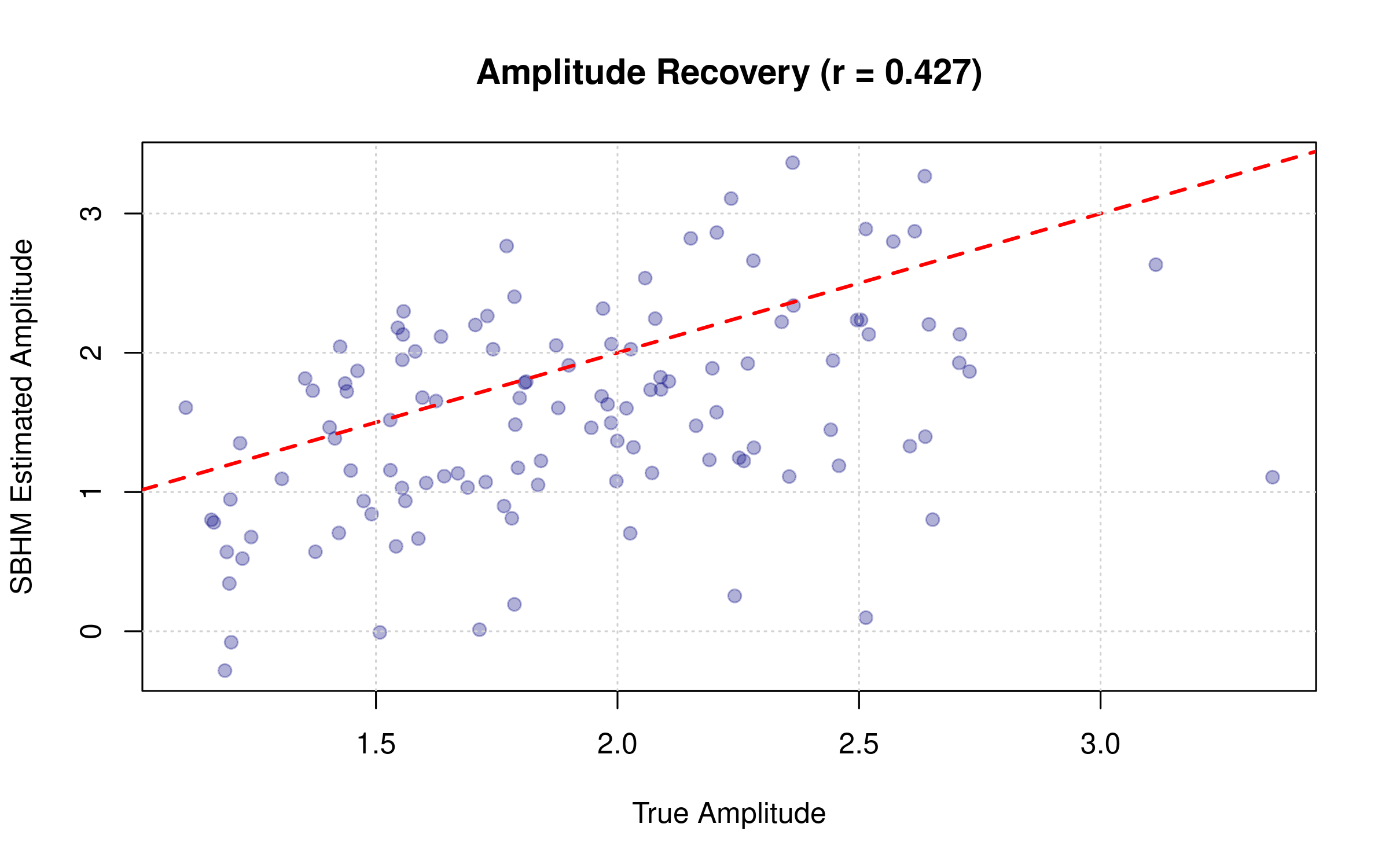

recovery_summary <- data.frame(
  HRFMatchingAccuracy = accuracy,
  AmplitudeCorrelation = cor_amp,
  MedianMargin = median(res_sbhm$margin)
)
recovery_summary
#>   HRFMatchingAccuracy AmplitudeCorrelation MedianMargin
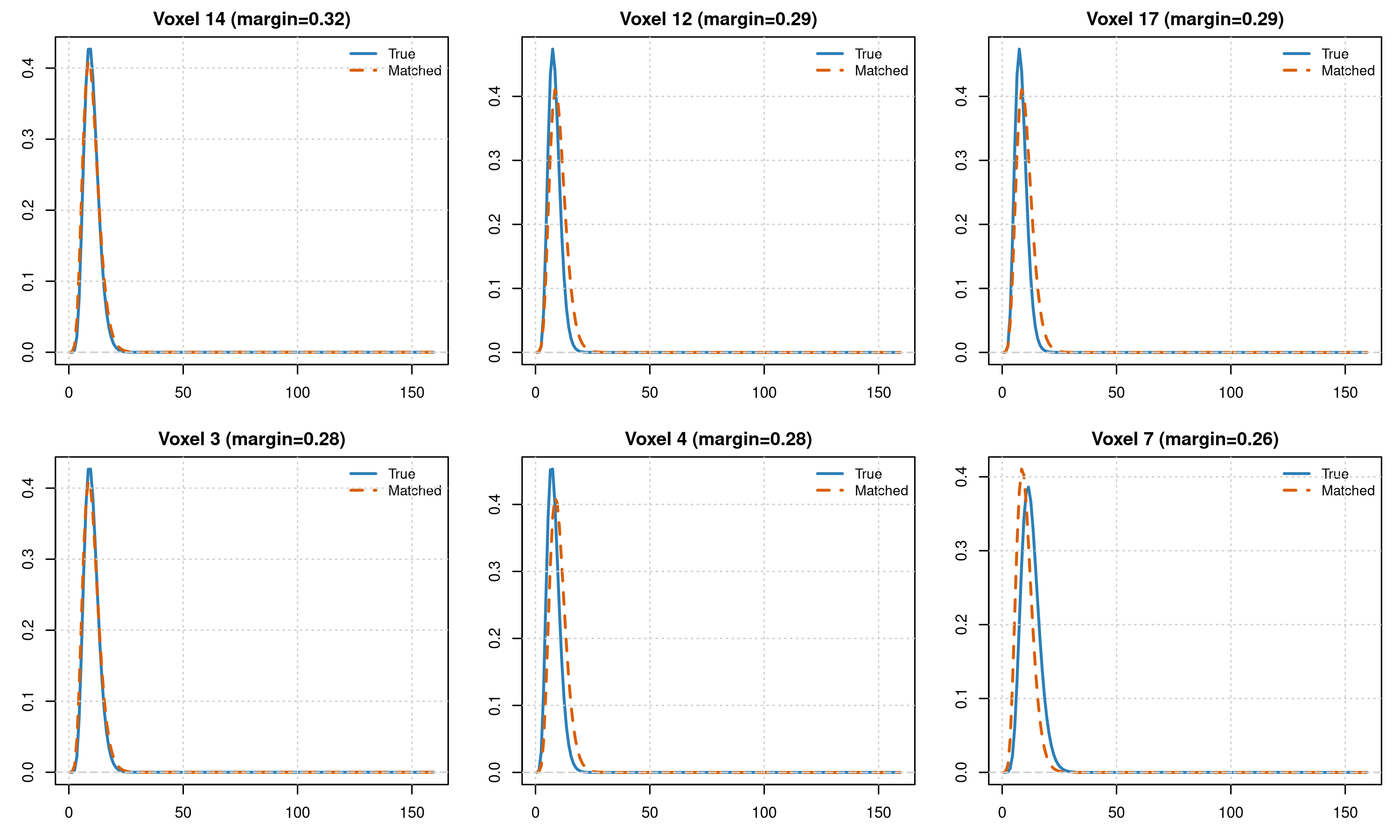
#> 1                0.75            0.6245209  0.005994378

Recovered HRF Shapes

For the most confidently matched voxels, the recovered and true HRFs should overlap closely.

H_hat <- sbhm$B %*% sbhm$A
vox_show <- head(order(-res_sbhm$margin), n = min(6, n_voxels))

par(mfrow = c(2, 3), mar = c(3, 3, 2, 1))
for (v in vox_show) {
  rng <- range(c(H_hat[, true_hrf_idx[v]], H_hat[, res_sbhm$matched_idx[v]]))
  plot(sbhm$tgrid, H_hat[, true_hrf_idx[v]], type = "l", col = "#2c7fb8",
       lwd = 2, ylim = rng, main = paste0("Voxel ", v), xlab = "Time (s)", ylab = "HRF")
  lines(sbhm$tgrid, H_hat[, res_sbhm$matched_idx[v]], col = "#d95f02", lwd = 2, lty = 2)
  legend("topright", bty = "n", cex = 0.8, legend = c("True", "Matched"),
         lty = 1:2, lwd = 2, col = c("#2c7fb8", "#d95f02"))
}

Library Manifold

PCA of the library coordinates shows which HRFs were present (true) versus selected (matched).

pca <- prcomp(t(sbhm$A), center = TRUE, scale. = TRUE)
pc <- pca$x[, 1:2, drop = FALSE]
plot(pc, pch = 16, col = "gray70", xlab = "PC1", ylab = "PC2",
     main = "Library Coordinate Space (PCA)")
points(pc[unique(true_hrf_idx), , drop = FALSE], pch = 1, col = "#2c7fb8", lwd = 2)
points(pc[unique(res_sbhm$matched_idx), , drop = FALSE], pch = 4, col = "#d95f02", lwd = 2)
legend("topright", bty = "n",
       legend = c("Library", "True", "Matched"),
       pch = c(16, 1, 4), col = c("gray60", "#2c7fb8", "#d95f02"))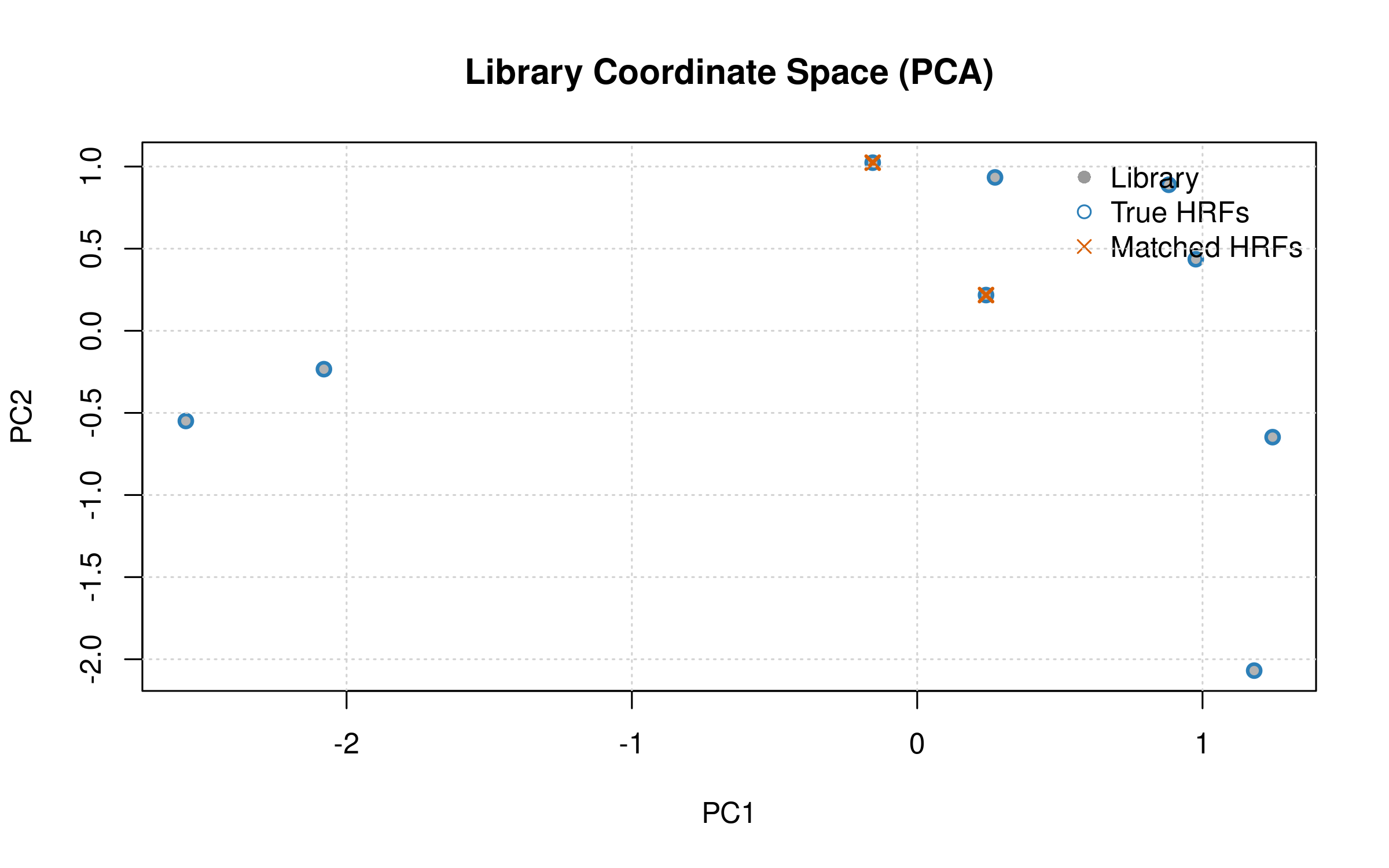

Soft Assignment for Ambiguous Voxels

Hard assignment picks the single best HRF per voxel. When the margin is small, blending the top-K candidates can reduce variance. The built-in approach requires just two extra arguments.

res_soft <- lss_sbhm(
  Y = Y, sbhm = sbhm, design_spec = design_spec,
  match = list(topK = 3, soft_blend = TRUE,
               blend_margin = median(res_sbhm$margin)),
  return = "amplitude"
)

cor_sv <- cor(as.vector(res_soft$amplitude), as.vector(res_sbhm$amplitude))
cat("Soft vs hard amplitude correlation:", round(cor_sv, 3), "\n")
#> Soft vs hard amplitude correlation: 0.994

Blending only applies to voxels whose margin falls below blend_margin; confident voxels keep their hard assignment. For manual control over the blending weights, use sbhm_prepass(), sbhm_match(topK = K), and sbhm_project() directly. See ?sbhm_match for details.

Shape Estimation Strategies

By default, SBHM estimates each voxel’s HRF shape from an aggregate prepass fit (alpha_source = "prepass"). Two alternative strategies are available when the prepass is unreliable:

• "trial_projection" estimates shape from per-trial projection coefficients in the shared basis, using the leading singular vector across trials.
• "oasis_rank1" extracts shape from the rank-1 approximation of the trial-wise OASIS betas. Set rank1_min to gate voxels with low rank-1 variance fraction back to prepass.

res_proj <- lss_sbhm(
  Y, sbhm, design_spec,
  match = list(alpha_source = "trial_projection")
)

Low-Confidence Gating

For voxels where matching is uncertain (low margin or weak signal), you can gate them to a fallback shape using min_margin and min_beta_norm. Gated voxels use the reference coordinate instead of the matched one.

res_gated <- lss_sbhm(
  Y, sbhm, design_spec,
  match = list(min_margin = 0.05, min_beta_norm = 1e-3)
)
cat("Voxels gated to fallback:", res_gated$diag$fallback_low_conf_n, "\n")

Amplitude Policy

The final amplitude stage estimates per-trial scalars from the matched HRF. The amplitude$method argument selects the estimator: "lss1" (default, per-trial 2x2 LSS—robust under overlap), "global_ls" (fast ridge-regularized GLM across all trials), or "oasis_voxel" (full OASIS per voxel, heaviest but returns SEs).

The default "lss1" provides the best balance of robustness and accuracy for typical rapid event-related designs. For slow designs with well-separated trials, "global_ls" can be faster. Use cond_gate to fall back automatically when the design is too collinear for a given method.

out <- lss_sbhm(
  Y, sbhm, design_spec,
  amplitude = list(method = "lss1",
                   ridge_frac = list(x = 0.02, b = 0.02),
                   cond_gate = list(metric = "rho", thr = 0.999, fallback = "global_ls"))
)

See ?lss_sbhm for guidance on choosing by ISI regime (slow, moderate, fast ER).

Returning Coefficients for Custom Analysis

When you need the full r-dimensional trial-wise coefficients instead of scalar amplitudes, request return = "coefficients".

res_c <- lss_sbhm(Y = Y[, 1:5], sbhm = sbhm,
                   design_spec = design_spec, return = "coefficients")
cat("Coefficients:", dim(res_c$coeffs_r), " [r x trials x voxels]\n")
#> Coefficients: 6 6 5  [r x trials x voxels]

Parameter Quick Reference

Parameter	Default	Recommended	Notes
r (rank)	–	6–12	Aim for 90–95% variance explained
topK	3	1–5	Use 3–5 with soft_blend = TRUE for ambiguous cases
soft_blend	TRUE	TRUE	Blend top-K candidates for uncertain voxels
blend_margin	0.08	0.05–0.15	Only blend voxels with margin below this
alpha_source	"prepass"	"prepass"	Also "trial_projection" or "oasis_rank1"
prepass$ridge	NULL	list(mode = "fractional", lambda = 0.01)	Stabilizes noisy/collinear designs
match$shrink$tau	0	0–0.2	Increase for low SNR
match$whiten	FALSE	FALSE	Set TRUE with whiten_power = 0.5 for partial whitening
match$min_margin	NULL	0.05–0.1	Gate low-confidence voxels to fallback shape
prewhiten	NULL	list(method = "ar", p = 1L)	Use for TR < 2s
amplitude$method	"lss1"	varies by ISI	"global_ls" for slow ER, "lss1" otherwise

For full details on every parameter, see ?sbhm_build, ?sbhm_match, and ?lss_sbhm.

Performance Considerations

SBHM’s cost scales as O(TrNV) for the LSS step, where N is the number of trials. Compared to unconstrained voxel-wise HRF estimation this is typically 10–50x faster, since r << KN.

For very large datasets (V > 50,000), PCA factorization reduces memory by fitting the prepass on q “meta-voxels” instead of V voxels.

pca_Y <- prcomp(Y, center = TRUE, rank. = 100)
res <- lss_sbhm(
  Y = pca_Y$x, sbhm = sbhm, design_spec = design_spec,
  prepass = list(data_fac = list(scores = pca_Y$x, loadings = pca_Y$rotation))
)

For ROI-based analyses, simply subset columns of Y before calling lss_sbhm(). A benchmark script is available via system.file("benchmarks", "bench_sbhm.R", package = "fmrilss").

Prewhitening

If your TR is short (< 2s) or residuals show autocorrelation, add prewhitening to the final OASIS step.

res_pw <- lss_sbhm(
  Y = Y, sbhm = sbhm, design_spec = design_spec,
  prewhiten = list(method = "ar", p = 1L, pooling = "global", exact_first = "ar1")
)

Note: the factorized prepass intentionally skips prewhitening for efficiency. The final OASIS step still applies it when prewhiten is provided.

References

• Mumford et al. (2012). “Deconvolving BOLD activation in event-related designs for multivoxel pattern classification analyses.” NeuroImage.
• Lindquist et al. (2009). “Modeling the hemodynamic response function in fMRI.” NeuroImage.

Summary

SBHM provides efficient, interpretable voxel-specific HRF estimation by learning a shared basis from a plausible library and matching each voxel in a low-dimensional coefficient space. The lss_sbhm() function runs the full pipeline in a single call, returning trial-wise amplitudes with per-voxel HRF assignments and confidence scores.

Next steps: see ?sbhm_build for library construction, ?lss_sbhm for the end-to-end pipeline, and the “Voxel-wise HRF” vignette for unconstrained alternatives.