Getting Started with fmrilss
fmrilss Development Team
2025-10-31
getting_started.RmdThe Challenge of Event-Related fMRI Analysis
In event-related fMRI experiments with rapid stimulus presentation, hemodynamic responses from consecutive trials overlap substantially due to the slow temporal dynamics of the BOLD signal (10-15 seconds). Traditional general linear models (GLMs) that estimate all trials simultaneously suffer from collinearity when inter-stimulus intervals are short (< 4 seconds), resulting in unstable trial-specific activation estimates. These unstable estimates compromise downstream analyses including multivariate pattern analysis (MVPA), representational similarity analysis (RSA), and trial-by-trial connectivity methods.
The Least Squares Separate (LSS) approach (Mumford et al., 2012)
addresses this collinearity problem by fitting a separate GLM for each
trial. In each model, one regressor represents the trial of interest
while a second regressor aggregates all other trials, reducing
collinearity and improving estimate stability. The fmrilss
package provides optimized implementations of LSS with extensions
including automatic HRF estimation, ridge regularization, and parallel
computation across multiple CPU cores.
Understanding the LSS Approach
This vignette assumes familiarity with fMRI general linear models, design matrices, hemodynamic response functions, and R matrix operations.
Standard GLM analysis (Least Squares All, LSA) estimates all trial coefficients simultaneously by solving: beta = (X’X)^(-1)X’Y. When trials occur in rapid succession, the design matrix columns exhibit high correlation (condition number > 30), producing unstable trial estimates with inflated variance.
LSS reformulates the problem by fitting N separate models, where N is the number of trials. For trial i, the design matrix contains: (1) a regressor for trial i, (2) a single regressor aggregating all other trials, and (3) any nuisance or baseline regressors. This reduces the effective condition number and produces more stable single-trial estimates. Mathematically, for trial i:
beta_i = (X_i’X_i)^(-1)X_i’Y
where X_i = [x_i | Σ(j≠i) x_j | Z | N], with x_i the trial regressor, Z experimental covariates, and N nuisance regressors.
Beyond these two core regressors, LSS models can include experimental regressors that capture session-wide effects like linear trends or block effects, which we want to model but don’t need trial-specific estimates for. The model can also incorporate nuisance regressors such as motion parameters or physiological noise, which are projected out before the analysis begins.
Your First LSS Analysis
The following example demonstrates LSS analysis using synthetic data from a rapid event-related design.
Creating the Experimental Design
The design matrix encodes stimulus timing and expected hemodynamic responses. We’ll create a proper event-related design by convolving trial onsets with an HRF.
# Define trial onsets (in TRs)
onsets <- round(seq(from = 10, to = n_timepoints - 12, length.out = n_trials))

# Create HRF-convolved design matrix using a simple gamma HRF
# In real analyses, use fmrihrf package for more sophisticated HRF models
simple_hrf <- function(t) {
  # Gamma function parameters for a canonical HRF shape
  ifelse(t >= 0, dgamma(t, shape = 6, rate = 1), 0)
}

# Build trial design matrix (X) with HRF convolution
X <- matrix(0, n_timepoints, n_trials)
hrf_kernel <- simple_hrf(0:20)  # HRF spanning ~20 TRs
for(i in 1:n_trials) {
  onset <- onsets[i]
  hrf_length <- min(length(hrf_kernel), n_timepoints - onset + 1)
  X[onset:(onset + hrf_length - 1), i] <- hrf_kernel[1:hrf_length]
}

# Experimental regressors (Z) - intercept and linear trend
# These are regressors we want to model but not trial-wise
Z <- cbind(Intercept = 1, LinearTrend = as.vector(scale(1:n_timepoints, center = TRUE, scale = FALSE)))

# Nuisance regressors - e.g., 6 motion parameters
Nuisance <- matrix(rnorm(n_timepoints * 6), n_timepoints, 6)
Matrix X contains HRF-convolved trial regressors. Matrix
Z contains experimental covariates (intercept and linear
trend). The nuisance matrix models unwanted variance (e.g., motion
parameters).
Visualizing Regressors
The following visualizations show experimental regressors (excluding intercept) and nuisance regressors, standardized for comparability.
Generating Realistic Data
Now we’ll create synthetic fMRI data that includes contributions from all these components, plus some noise to make it realistic:
# Simulate effects for each component
true_trial_betas <- matrix(rnorm(n_trials * n_voxels, 0, 1.2), n_trials, n_voxels)
true_fixed_effects <- matrix(rnorm(2 * n_voxels, c(5, -0.1), 0.5), 2, n_voxels)
true_nuisance_effects <- matrix(rnorm(6 * n_voxels, 0, 2), 6, n_voxels)

# Combine signals and add noise
Y <- (Z %*% true_fixed_effects) +
     (X %*% true_trial_betas) +
     (Nuisance %*% true_nuisance_effects) +
     matrix(rnorm(n_timepoints * n_voxels, 0, 1), n_timepoints, n_voxels)
Running the Analysis
The lss() function provides a clean, modern interface
that adapts to your needs. At its simplest, you can provide just the
data and trial matrix, and the function automatically includes an
intercept term:
For a more complete analysis that accounts for experimental effects
and removes nuisance signals, we include our Z and
Nuisance matrices. The function handles the nuisance
regression efficiently, projecting these signals out of both the data
and design matrix before estimating trial-specific betas:
Handling Temporal Autocorrelation with Prewhitening
fMRI time series exhibit temporal autocorrelation that can affect
statistical inference. The fmrilss package now integrates
with fmriAR to provide sophisticated prewhitening
capabilities:
# Basic AR(1) prewhitening
beta_ar1 <- lss(Y, X, Z = Z, Nuisance = Nuisance,
                prewhiten = list(method = "ar", p = 1))

# Automatic AR order selection
beta_auto <- lss(Y, X, Z = Z, Nuisance = Nuisance,
                prewhiten = list(method = "ar", p = "auto", p_max = 4))

# The prewhitened estimates account for temporal dependencies
dim(beta_ar1)
#> [1] 12 25
For more advanced noise modeling, you can use voxel-specific parameters or ARMA models:
# Voxel-specific AR parameters (slower but more accurate)
# Default pooling="global" estimates one AR model across all voxels
# pooling="voxel" fits separate AR models per voxel (~100x slower)
beta_voxel <- lss(Y, X, Z = Z, Nuisance = Nuisance,
                  prewhiten = list(method = "ar", p = 1, pooling = "voxel"))

# ARMA model for complex noise (AR + moving average components)
# Use when residuals show both autocorrelation and moving average patterns
beta_arma <- lss(Y, X, Z = Z, Nuisance = Nuisance,
                prewhiten = list(method = "arma", p = 2, q = 1))
Pooling strategies: -
pooling = "global" (default): Single AR model for all
voxels (fast) - pooling = "voxel": Per-voxel AR models
(accurate but slow) - pooling = "run": Separate model per
run (for multi-run data)
Choosing the Right Computational Backend
The fmrilss package offers multiple computational
backends, each optimized for different scenarios. While the default R
implementation is well-optimized and readable, making it excellent for
understanding the algorithm and debugging, you’ll often want to use the
high-performance C++ backend for real analyses, especially with large
datasets. The C++ implementation leverages Armadillo for efficient
linear algebra and OpenMP for parallel processing across multiple CPU
cores:
# Run the same analysis with the high-performance C++ engine
beta_fast <- lss(Y, X, Z = Z, Nuisance = Nuisance, method = "cpp_optimized")

# The results are numerically identical to the R version
all.equal(beta_full, beta_fast, tolerance = 1e-8)
#> [1] TRUE

# Combine prewhitening with fast computation
beta_fast_ar <- lss(Y, X, Z = Z, Nuisance = Nuisance,
                    method = "cpp_optimized",
                    prewhiten = list(method = "ar", p = 1))
This modular design allows seamless switching between backends without code changes. The R implementation facilitates debugging and development, while the C++ version provides production performance.
LSS versus Traditional GLM: When Each Shines
Comparison between LSS and standard Least Squares All (LSA) methods. LSA is the traditional GLM approach that estimates all trial coefficients simultaneously in a single model, making it computationally faster but more susceptible to collinearity in rapid designs.
# LSA: Standard GLM (Least Squares All) estimates all trials simultaneously
# This is computationally faster but suffers from collinearity in rapid designs
beta_lsa <- lsa(Y, X, Z = Z, Nuisance = Nuisance)

# Compare dimensions
cat("LSS beta dimensions:", dim(beta_full), "\n")
#> LSS beta dimensions: 12 25
cat("LSA beta dimensions:", dim(beta_lsa), "\n")
#> LSA beta dimensions: 12 25

# Compare variance in beta estimates
var_lss <- apply(beta_full, 2, var)
var_lsa <- apply(beta_lsa, 2, var)

cat("\nMean variance across voxels:\n")
#>
#> Mean variance across voxels:
cat("  LSS:", mean(var_lss), "\n")
#>   LSS: 10.27741
cat("  LSA:", mean(var_lsa), "\n")
#>   LSA: 195.8418

# Plot comparison
par(mfrow = c(1, 2))
hist(beta_full[, 1], main = "LSS: Beta distribution (Voxel 1)",
     xlab = "Beta values", col = "lightblue")
hist(beta_lsa[, 1], main = "LSA: Beta distribution (Voxel 1)",
     xlab = "Beta values", col = "lightgreen")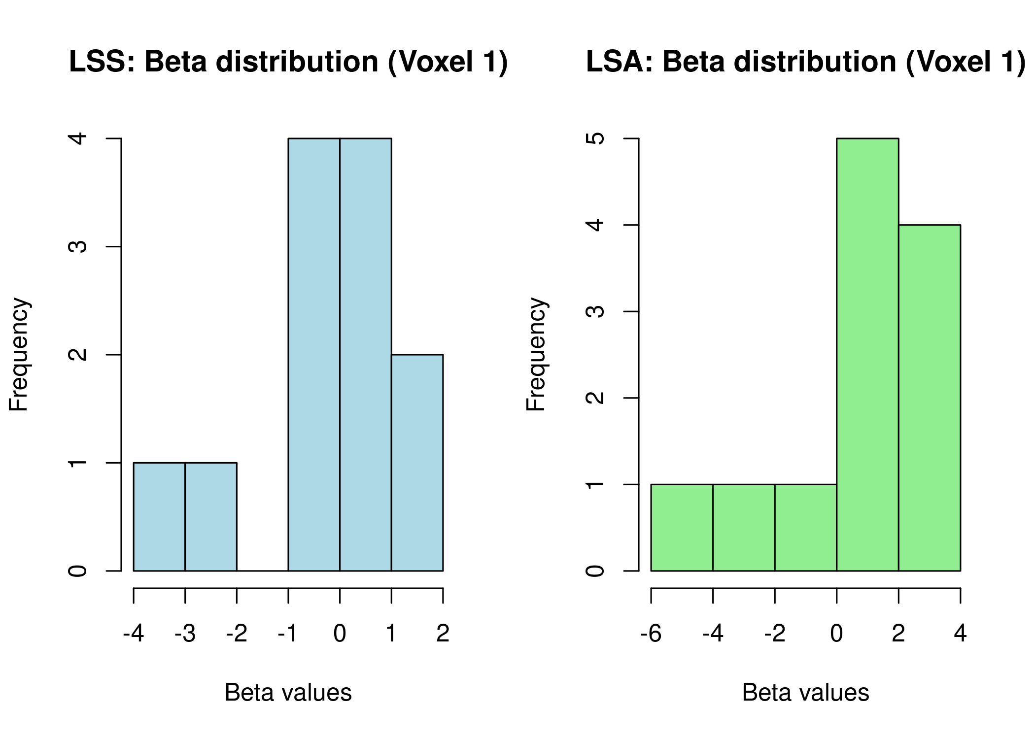
LSS produces beta estimates with different variance characteristics than LSA. Method selection criteria:
Use LSS for: - MVPA and pattern classification analyses - Rapid event-related designs (ISI < 4 seconds) - Trial-by-trial connectivity analyses - Representational similarity analysis (RSA)
Use LSA for: - Block designs with well-separated trials - Group-level contrast estimation - Designs with ISI > 6 seconds - When computational efficiency is critical
Introducing the OASIS Method
The OASIS (Optimized Analytic Single-pass Inverse Solution) method extends LSS with: automatic HRF estimation, ridge regularization for stability, single-pass computation for all trials, and multi-basis HRF model support.
# Basic OASIS usage with automatic design construction
# fmrihrf is now imported automatically
beta_oasis <- lss(
  Y = Y,
  X = NULL,  # Let OASIS build design from design_spec
  method = "oasis",
  oasis = list(
    design_spec = list(
      sframe = sampling_frame(blocklens = nrow(Y), TR = 1),
      cond = list(
        onsets = onsets,        # reuse onsets from above
        hrf = HRF_SPMG1,        # SPM canonical HRF
        span = 30               # HRF duration in seconds
      )
    ),
    ridge_mode = "fractional",  # Regularization for numerical stability
    ridge_x = 0.01,             # Ridge for design matrix
    ridge_b = 0.01              # Ridge for coefficients
  )
)

cat("OASIS beta dimensions:", dim(beta_oasis), "\n")
#> OASIS beta dimensions: 12 25

# Alternative: Provide a pre-built design matrix directly
# beta_oasis_manual <- lss(Y, X = my_hrf_convolved_design, method = "oasis", ...)
Why X = NULL? OASIS can build the
design matrix internally from design_spec, ensuring the HRF
settings stay synchronized with the design. This is especially useful
when exploring different HRFs or using multi-basis models.
Alternatively, you can provide your own HRF-convolved design via
X.
Working with Different Computational Backends
The package provides multiple backends to match your computational
needs and resources. Each backend implements the same algorithm but with
different optimization strategies. The naive implementation
offers the clearest code for understanding the algorithm, while
r_vectorized and r_optimized provide good
performance with pure R code. For production work with large datasets,
cpp_optimized offers the best performance, especially when
combined with parallel processing.
# Benchmark different methods
library(microbenchmark)

methods <- c("naive", "r_vectorized", "r_optimized", "cpp_optimized")
timings <- list()

for (m in methods) {
  timings[[m]] <- system.time({
    lss(Y, X, method = m)
  })[3]
}

# Display timing comparison
timing_df <- data.frame(
  Method = methods,
  Time = unlist(timings)
)
print(timing_df)

# For large datasets, consider threading for C++ backends
if (require("parallel")) {
  n_cores <- parallel::detectCores() - 1
  # Set OpenMP threads for C++ backend if supported
  Sys.setenv(OMP_NUM_THREADS = n_cores)
}
Handling Complex Experimental Designs
Real experiments often involve multiple conditions, parametric
modulations, and various covariates. The fmrilss package
handles these complexities gracefully. When working with multiple
conditions, you can create separate design matrices for each condition
and include condition labels as experimental regressors. This allows you
to model condition-specific effects while still obtaining trial-wise
estimates within each condition.
# Create design with multiple conditions
n_cond <- 3
X_multi <- matrix(0, n_timepoints, n_trials * n_cond)

# Generate a simple HRF for demonstration
hrf <- c(0, 0.2, 0.5, 0.8, 1, 0.9, 0.7, 0.5, 0.3, 0.1)

for (c in 1:n_cond) {
  trial_idx <- ((c-1) * n_trials + 1):(c * n_trials)
  for (i in 1:n_trials) {
    onset <- 10 + (trial_idx[i] - 1) * 5
    if (onset + 9 <= n_timepoints) {
      X_multi[onset:(onset + 9), trial_idx[i]] <- hrf
    }
  }
}

# Add condition labels as experimental regressors
Z_cond <- matrix(0, n_timepoints, n_cond)
for (c in 1:n_cond) {
  trial_idx <- ((c-1) * n_trials + 1):(c * n_trials)
  Z_cond[, c] <- rowSums(X_multi[, trial_idx, drop = FALSE])
}

# Run LSS with condition regressors
beta_multi <- lss(Y, X_multi, Z = Z_cond, method = "r_optimized")
Parametric modulations, where trial responses are weighted by continuous variables like reaction time or stimulus intensity, are also straightforward to implement. For a quantitative demo, we simulate a parametric effect in the data and show recovery with and without the modulator:
# Add parametric modulator (e.g., reaction time, stimulus intensity)
modulator <- scale(rnorm(n_trials, mean = 0, sd = 1), center = TRUE, scale = FALSE)

# Create parametrically modulated design (scale each trial by its modulator)
X_param <- sweep(X, 2, as.numeric(modulator), `*`)

# Simulate data with a parametric effect (reuse fixed and nuisance parts)
Y_mod <- (Z %*% true_fixed_effects) +
         (X_param %*% true_trial_betas) +
         (Nuisance %*% true_nuisance_effects) +
         matrix(rnorm(n_timepoints * n_voxels, 0, 1), n_timepoints, n_voxels)

# Fit models with and without the parametric modulator
beta_unmod <- lss(Y_mod, X,       Z = Z, method = "r_optimized")
beta_param <- lss(Y_mod, X_param, Z = Z, method = "r_optimized")

# Ground truth depends on which design matrix we use:
# - When fitting with X (unmodulated):        recovers modulator * true_trial_betas
# - When fitting with X_param (premodulated): recovers true_trial_betas directly
true_unmod_coefs <- sweep(true_trial_betas, 1, as.numeric(modulator), `*`)

cor_unmod <- cor(as.vector(beta_unmod), as.vector(true_unmod_coefs))
cor_param <- cor(as.vector(beta_param), as.vector(true_trial_betas))

cat("Correlation with true coefficients (parametric effect simulated):\n")
#> Correlation with true coefficients (parametric effect simulated):
cat("  Using X (no modulator):\t", round(cor_unmod, 3), "\n")
#>   Using X (no modulator):     0.138
cat("  Using X_param (with modulator):", round(cor_param, 3), "\n")
#>   Using X_param (with modulator): 0.103
Optimizing Performance for Large-Scale Analyses
When working with whole-brain data containing hundreds of thousands of voxels, memory management and computational efficiency become critical. The package provides several strategies for handling large datasets effectively.
For very large datasets that exceed available memory, you can process voxels in chunks. This approach maintains reasonable memory usage while still benefiting from vectorized operations within each chunk:
# For very large datasets, process in chunks
chunk_size <- 1000
n_chunks <- ceiling(ncol(Y) / chunk_size)

beta_chunks <- list()
for (chunk in 1:n_chunks) {
  voxel_idx <- ((chunk - 1) * chunk_size + 1):min(chunk * chunk_size, ncol(Y))
  beta_chunks[[chunk]] <- lss(Y[, voxel_idx], X, method = "cpp_optimized")
}

# Combine results
beta_full <- do.call(cbind, beta_chunks)
Another optimization strategy involves preprocessing your data to remove nuisance signals before running LSS. While LSS can handle nuisance regressors internally, preprocessing can be more efficient when running multiple analyses:
# Project out nuisance before LSS (when appropriate)
# project_confounds returns the projection matrix Q; apply it to both Y and X
Q_nuis <- project_confounds(Nuisance)
Y_clean <- Q_nuis %*% Y
X_clean <- Q_nuis %*% X

# This can be faster than including Nuisance in each LSS iteration
beta_preprocessed <- lss(Y_clean, X_clean, Z = Z, method = "r_optimized")
Choosing the right backend for your data size is crucial for optimal performance:
Performance guidelines (based on benchmarks):
| Data Size | Recommended Method | Rationale |
|---|---|---|
| n_trials < 50, n_voxels < 5,000 |
r_optimized or cpp_optimized
|
Similar speed, R easier to debug |
| n_voxels > 10,000 | cpp_optimized |
Benefits from OpenMP parallelization |
| Need HRF grid search or ridge | oasis |
Additional features justify overhead |
| Quick prototyping | r_optimized |
Good balance of speed and readability |
In practice, pick the backend that matches your needs: R for debugging, C++ for maximum throughput, OASIS for HRF-aware workflows. Always validate with a quick benchmark on your own data.
Troubleshooting Common Challenges
Even with robust implementations, certain data characteristics can cause issues. Understanding how to diagnose and address these problems will help you get the most out of your analyses.
When design matrices become singular or near-singular due to high collinearity between regressors, standard least squares solutions become unstable. You can detect this by examining the correlation matrix of your design:
# Check for collinearity in design matrix
cor_matrix <- cor(X)
high_cor <- which(abs(cor_matrix) > 0.9 & cor_matrix != 1, arr.ind = TRUE)

if (nrow(high_cor) > 0) {
  warning("High correlation between regressors detected")

  # Option 1: Use OASIS with ridge and automatic design construction
  beta_ridge <- lss(
    Y = Y,
    X = NULL,  # Let OASIS build design
    method = "oasis",
    oasis = list(
      design_spec = list(
        sframe = sampling_frame(blocklens = nrow(Y), TR = 1),
        cond = list(onsets = onsets, hrf = HRF_SPMG1, span = 30)
      ),
      ridge_mode = "absolute",
      ridge_x = 0.1  # Stronger ridge for collinearity
    )
  )

  # Option 2: For standard LSS without OASIS, increase ISI or use prewhitening
  # Ridge is not directly available for non-OASIS backends
}
Memory limitations can also pose challenges with large datasets. Before starting an analysis, it’s wise to estimate memory requirements and adjust your approach accordingly:
# Estimate peak memory requirements
mem_Y <- object.size(Y)
mem_designs_approx <- mem_Y * n_trials  # n_trials copies of design during LSS
mem_results <- mem_Y  # Output size similar to Y
mem_required <- mem_Y + mem_designs_approx + mem_results

cat("Estimated memory needed:", round(mem_required / 1e9, 2), "GB\n")

# If this exceeds available RAM, use chunking approach (see example above)
# Or consider OASIS which has lower memory overhead for large datasets
If you encounter unexpectedly slow performance, profiling can help identify bottlenecks:
# Profile code to find bottlenecks
Rprof("lss_profile.out")
beta_slow <- lss(Y, X, method = "naive")
Rprof(NULL)
summaryRprof("lss_profile.out")
Where to Go From Here
This vignette has introduced you to the core concepts and
capabilities of the fmrilss package. You’ve learned how LSS
addresses the collinearity problem in rapid event-related designs, how
to choose between different computational backends, and strategies for
handling complex experimental designs and large datasets.
To deepen your understanding and explore advanced features, we recommend:
- Voxel-wise HRF vignette: Model spatial variation in hemodynamic responses across the brain using fully flexible HRF estimation
- SBHM vignette: Learn efficient voxel-specific HRF estimation using Shared-Basis HRF Matching, a library-constrained approach that balances flexibility and computational efficiency
- OASIS method vignette: Comprehensive coverage of OASIS features including automatic HRF construction, ridge regularization, and multi-basis models
- Mixed models vignette: Combine LSS with mixed-effects modeling frameworks for hierarchical analyses
The fmrilss package represents a comprehensive toolkit
for trial-wise beta estimation, providing options that range from
simple, interpretable implementations to highly optimized solutions for
large-scale analyses. Whether you’re conducting exploratory analyses on
a laptop or processing massive datasets on a computing cluster, the
package offers the flexibility and performance you need for modern fMRI
analysis.
References
Mumford, J. A., Turner, B. O., Ashby, F. G., & Poldrack, R. A. (2012). Deconvolving BOLD activation in event-related designs for multivoxel pattern classification analyses. NeuroImage, 59(3), 2636-2643.
Session Info
#> R version 4.5.1 (2025-06-13)
#> Platform: x86_64-pc-linux-gnu
#> Running under: Ubuntu 24.04.3 LTS
#>
#> Matrix products: default
#> BLAS:   /usr/lib/x86_64-linux-gnu/openblas-pthread/libblas.so.3
#> LAPACK: /usr/lib/x86_64-linux-gnu/openblas-pthread/libopenblasp-r0.3.26.so;  LAPACK version 3.12.0
#>
#> locale:
#>  [1] LC_CTYPE=C.UTF-8       LC_NUMERIC=C           LC_TIME=C.UTF-8
#>  [4] LC_COLLATE=C.UTF-8     LC_MONETARY=C.UTF-8    LC_MESSAGES=C.UTF-8
#>  [7] LC_PAPER=C.UTF-8       LC_NAME=C              LC_ADDRESS=C
#> [10] LC_TELEPHONE=C         LC_MEASUREMENT=C.UTF-8 LC_IDENTIFICATION=C
#>
#> time zone: UTC
#> tzcode source: system (glibc)
#>
#> attached base packages:
#> [1] stats     graphics  grDevices utils     datasets  methods   base
#>
#> other attached packages:
#> [1] fmrilss_0.1.0          fmrihrf_0.1.0.9000     RcppArmadillo_15.0.2-2
#> [4] Rcpp_1.1.0
#>
#> loaded via a namespace (and not attached):
#>  [1] Matrix_1.7-3        gtable_0.3.6        jsonlite_2.0.0
#>  [4] compiler_4.5.1      assertthat_0.2.1    jquerylib_0.1.4
#>  [7] splines_4.5.1       systemfonts_1.3.1   scales_1.4.0
#> [10] textshaping_1.0.4   uuid_1.2-1          yaml_2.3.10
#> [13] fastmap_1.2.0       lattice_0.22-7      ggplot2_4.0.0
#> [16] R6_2.6.1            knitr_1.50          desc_1.4.3
#> [19] RColorBrewer_1.1-3  bslib_0.9.0         rlang_1.1.6
#> [22] cachem_1.1.0        xfun_0.53           S7_0.2.0
#> [25] fs_1.6.6            sass_0.4.10         memoise_2.0.1
#> [28] cli_3.6.5           pkgdown_2.1.3       magrittr_2.0.4
#> [31] digest_0.6.37       grid_4.5.1          bigmemory.sri_0.1.8
#> [34] lifecycle_1.0.4     bigmemory_4.6.4     vctrs_0.6.5
#> [37] evaluate_1.0.5      glue_1.8.0          farver_2.1.2
#> [40] numDeriv_2016.8-1.1 fmriAR_0.1.0        ragg_1.5.0
#> [43] rmarkdown_2.30      purrr_1.1.0         tools_4.5.1
#> [46] htmltools_0.5.8.1