Generic function to evaluate a regressor object over a specified time grid. Different types of regressors may have different evaluation methods.
Usage
evaluate(x, grid, ...)

# S3 method for class 'Reg'
evaluate(
  x,
  grid,
  precision = 0.33,
  method = c("conv", "loop", "fft", "Rconv"),
  sparse = FALSE,
  normalize = FALSE,
  ...
)
Arguments
- x
A `Reg` object (or an object inheriting from it, like `regressor`).
- grid
Numeric vector specifying the time points (seconds) for evaluation.
- ...
Additional arguments passed down (e.g., to `evaluate.HRF` in the loop method).
- precision
Numeric sampling precision for internal HRF evaluation and convolution (seconds).
- method
The evaluation method:
- conv
(Default, recommended) C++ direct convolution. Fastest in every configuration benchmarked – typically 3-10x faster than `fft` and 10-100x faster than `loop` – and accurate to ~1e-3 relative against numerical integration of the same design.
- loop
Pure R, evaluating the HRF at exact per-event relative times. Roughly twice as accurate as `conv` because event onsets are never quantised to the internal grid, but far slower. Retained as a reference implementation, and used automatically when `hrf` is a list of per-event HRFs.
- fft
Deprecated. The HRF is short relative to the sampled design, so an FFT never repaid its zero-padding; it was also the only method that could fail outright, on an internal FFT size above ~1e7. Now evaluates via `conv` and warns.
- Rconv
Deprecated. An R reimplementation of `conv` that required a regular grid and constant durations and silently fell back to `loop` otherwise. Now evaluates via `conv` and warns.
- sparse
Logical indicating whether to return a sparse matrix (from the Matrix package). Default is FALSE.
- normalize
Logical; if TRUE, scale evaluated regressor output to unit peak (maximum absolute value of 1). For multi-basis regressors, each basis column is normalized independently.
Examples
# Create a regressor
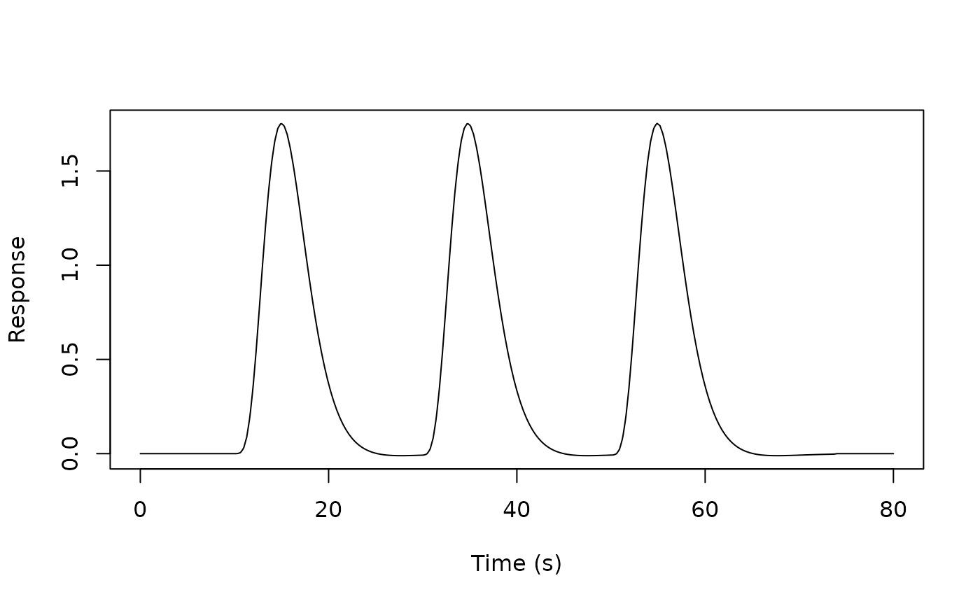
reg <- regressor(onsets = c(10, 30, 50), hrf = HRF_SPMG1)
# Evaluate at specific time points
times <- seq(0, 80, by = 0.1)
response <- evaluate(reg, times)
# Plot the response
plot(times, response, type = "l", xlab = "Time (s)", ylab = "Response")
 # Create a regressor
reg <- regressor(onsets = c(10, 30, 50), hrf = HRF_SPMG1)
# Evaluate with default method (conv)
times <- seq(0, 80, by = 0.5)
response <- evaluate(reg, times)
# Try different evaluation methods
response_loop <- evaluate(reg, times, method = "loop")
# With higher precision
response_precise <- evaluate(reg, times, precision = 0.1)
# Create a regressor
reg <- regressor(onsets = c(10, 30, 50), hrf = HRF_SPMG1)
# Evaluate with default method (conv)
times <- seq(0, 80, by = 0.5)
response <- evaluate(reg, times)
# Try different evaluation methods
response_loop <- evaluate(reg, times, method = "loop")
# With higher precision
response_precise <- evaluate(reg, times, precision = 0.1)