OASIS Theory: Algebra and Implementation Details

fmrilss Development Team

2025-09-29

Motivation

Optimized Analytic Single-pass Inverse Solution (OASIS) extends Least Squares Separate (LSS) estimation through algebraic reformulation that enables single-pass computation of all trial estimates. For a single-basis HRF (K = 1) without ridge, OASIS reduces exactly to the closed-form LSS solution; the per‑trial 2x2 normal equations are the same. The value of OASIS is in batching those solves efficiently and generalizing the same algebra to multi‑basis HRFs (2Kx2K) with optional ridge and diagnostics. This document provides the mathematical foundation and implementation details.

Computational Intuition

Standard LSS requires N separate GLM fits for N trials, each involving: 1. Matrix assembly: O(T²) operations 2. QR decomposition: O(T³) operations 3. Back-substitution: O(T²) operations

Total complexity: O(NT³) for N trials

OASIS recognizes that these N models share substantial structure. By factoring out common computations, OASIS reduces complexity to: 1. Single QR decomposition: O(T³) 2. Shared projections: O(NT²) 3. Per-trial solutions: O(N)

Total complexity: O(T³ + NT²), a significant reduction when N is large.

Visual Comparison of Computational Scaling

# Demonstrate computational scaling
N_trials <- c(10, 50, 100, 200, 500, 1000)
T_points <- 200  # Fixed number of timepoints

# Simplified complexity models (arbitrary units)
classical_ops <- N_trials * T_points^3 / 1e6  # O(NT³)
oasis_ops <- (T_points^3 + N_trials * T_points^2) / 1e6  # O(T³ + NT²)

# Create comparison plot
plot(N_trials, classical_ops, type='l', col='red', lwd=2,
     xlab='Number of Trials', ylab='Computational Operations (millions)',
     main='Computational Complexity: Classical LSS vs OASIS',
     ylim=c(0, max(classical_ops)))
lines(N_trials, oasis_ops, col='blue', lwd=2)
legend('topleft', c('Classical LSS', 'OASIS'),
       col=c('red', 'blue'), lwd=2, bty='n')

# Add shaded region showing computational savings
polygon(c(N_trials, rev(N_trials)),
        c(classical_ops, rev(oasis_ops)),
        col=rgb(0.2, 0.8, 0.2, 0.3), border=NA)
text(500, mean(c(classical_ops[4], oasis_ops[4])),
     'Computational\nSavings', col='darkgreen')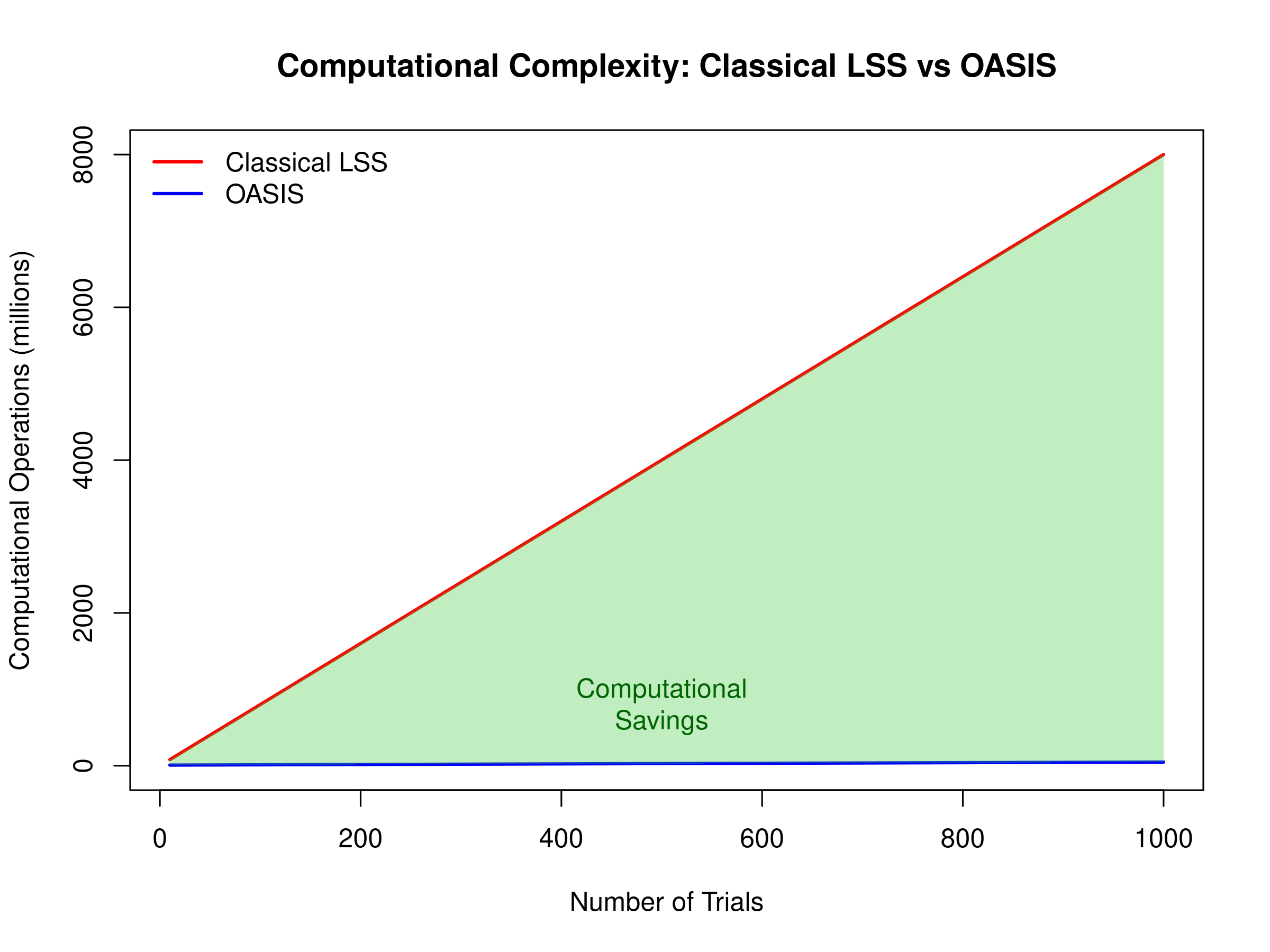

Computational complexity: Classical LSS vs OASIS

Prerequisites

This vignette assumes familiarity with: - QR decomposition and orthogonal projection matrices - Ridge regression and regularization - Matrix calculus and linear algebra - The standard LSS formulation

Code references point to R/oasis_glue.R and src/oasis_core.cpp implementations.

Notation used throughout:

• $Y \in \mathbb{R}^{T \times V}$: voxel data ($T$ time points, $V$ voxels)
• $X = [x_1, \dots, x_N] \in \mathbb{R}^{T \times N}$: trial regressors for one condition
• $Z \in \mathbb{R}^{T \times K_z}$: nuisance/experimental regressors shared across trials
• $R = I - QQ^T$: orthogonal projector removing nuisance effects ($Q$ comes from QR factorisation of $[Z,\text{others}]$)
• Inner products are denoted $\langle a, b \rangle = a^T b$

We first treat the single-basis case (one regressor per trial) before generalizing to multi-basis HRFs.

Classical LSS Recap

Classical LSS fits, for each trial $j$, a GLM with design $[x_j, b_j, Z]$, where $b_j = \sum_{i \neq j} x_i$. Solving each model independently costs $\mathcal{O}(N)$ QR factorizations. Algebraically, the trial-specific beta can be expressed as

$$\hat{\beta}_j = \frac{\langle Rx_j, RY \rangle - \frac{\langle Rx_j, Rb_j \rangle}{\|Rb_j\|^2} \langle Rb_j, RY \rangle}{\|Rx_j\|^2 - \frac{\langle Rx_j, Rb_j \rangle^2}{\|Rb_j\|^2}}.$$

OASIS extracts and reuses the common computational components (projections, norms, cross-products) across all trials, computing each only once.

Single-Basis OASIS Algebra

After residualising against nuisance regressors we define:

• $a_j = Rx_j$
• $s = \sum_{j=1}^N a_j$
• $d_j = \|a_j\|^2$
• $\alpha_j = \langle a_j, s - a_j \rangle$
• $s_j = \|s - a_j\|^2$

Let $n_{jv} = \langle a_j, RY_{\cdot v} \rangle$ and $m_v = \langle s, RY_{\cdot v} \rangle$. The pair $(\beta_j, \gamma_j)$ solving the 2x2 system for trial $j$ and voxel $v$ is obtained from

$$G_j \begin{bmatrix} \beta_{jv} \\ \gamma_{jv} \end{bmatrix} = \begin{bmatrix} n_{jv} \\ m_v - n_{jv} \end{bmatrix}, \quad G_j = \begin{bmatrix} d_j + \lambda_x & \alpha_j \\ \alpha_j & s_j + \lambda_b \end{bmatrix},$$

with ridge penalties $\lambda_x, \lambda_b \ge 0$. The inverse of $G_j$ is analytic, so
$$\beta_{jv} = \frac{(s_j + \lambda_b) n_{jv} - \alpha_j (m_v - n_{jv})}{(d_j + \lambda_x)(s_j + \lambda_b) - \alpha_j^2}.$$

This is exactly what oasis_betas_closed_form() implements (C++ file src/oasis_core.cpp). The precomputation step oasis_precompute_design() produces $a_j, s, d_j, \alpha_j, s_j$ once, while oasis_AtY_SY_blocked() streams through voxels to obtain $n_{jv}$ and $m_v$.

Fractional Ridge

oasis$ridge_mode = "fractional" sets $\lambda_x = \eta_x \cdot \bar{d}$ and $\lambda_b = \eta_b \cdot \bar{s}$, where $\bar{d}$ and $\bar{s}$ are means of $d_j$ and $s_j$. The helper .oasis_resolve_ridge() implements this scaling. Absolute ridge uses the supplied values directly.

Standard Errors

Given $G_j^{-1}$ and residual norm $\|RY\|^2$, the variance of $\beta_{jv}$ is

$$\operatorname{Var}(\hat{\beta}_{jv}) = \sigma_{jv}^2 \left( G_j^{-1} \right)_{11}, \quad \sigma_{jv}^2 = \frac{\text{SSE}_{jv}}{\text{dof}},$$

with

$$\text{SSE}_{jv} = \|RY_{\cdot v}\|^2 - 2 (\beta_{jv} n_{jv} + \gamma_{jv} (m_v - n_{jv})) + d_j \beta_{jv}^2 + s_j \gamma_{jv}^2 + 2 \alpha_j \beta_{jv} \gamma_{jv}.$$

.oasis_se_from_norms() realises this computation, reusing $n_{jv}$, $m_v$ and the cached design scalars.

Multi-Basis Extension

When the HRF contributes $K > 1$ basis functions, each trial has columns $A_j \in \mathbb{R}^{T \times K}$. Define

• $S = \sum_j A_j$
• $D_j = A_j^T A_j$
• $C_j = A_j^T (S - A_j)$
• $E_j = (S - A_j)^T (S - A_j)$

Per voxel we need $N1 = A^T RY$ (stacked $N$ blocks of size $K$) and $SY = S^T RY$. The block system is

$$\begin{bmatrix} D_j + \lambda_x I & C_j \\ C_j^T & E_j + \lambda_b I \end{bmatrix} \begin{bmatrix} B_{jv} \\ \Gamma_{jv} \end{bmatrix} = \begin{bmatrix} N1_{jv} \\ SY_v - N1_{jv} \end{bmatrix},$$

where $B_{jv} \in \mathbb{R}^K$. oasisk_betas() solves this 2Kx2K system via Cholesky factorisation. Ridge again adds $\lambda_x I$ and $\lambda_b I$ to the block diagonals. Compared to the single-basis path, only the shapes of the cached matrices differ; the solve is still analytic per trial/voxel block.

The companion oasisk_betas_se() extends the SSE/variance calculation to the multi-basis case, using the same building blocks.

HRF-Aware Design Construction

OASIS can construct $X$ on the fly from event specifications. .oasis_build_X_from_events() uses fmrihrf::regressor_set() to generate trial-wise columns (and optional other-condition aggregates) given:

• cond$onsets: per-trial onset times
• cond$hrf: HRF object (canonical, FIR, multi-basis, user-defined)
• cond$span, precision, method: convolution controls

This design is then residualised against nuisance regressors and fed into the algebra above. Because the HRF definition enters directly, switching HRFs or running grid searches automatically regenerates a matching design. When you provide an explicit X, OASIS skips this step and assumes you have already encoded the HRF in the matrix.

AR(1) Whitening

oasis$whiten = "ar1" estimates a common AR(1) coefficient from residualised data. .oasis_ar1_whitener() computes $\rho$ and applies Toeplitz-safe differencing:

$$\tilde{y}_t = \begin{cases} \sqrt{1 - \rho^2} y_1 & t = 1, \\ y_t - \rho y_{t-1} & t > 1. \end{cases}$$

The same transformation is applied to $X$ and nuisance regressors before the standard OASIS algebra runs. Whitening preserves the single-pass benefits because the transformed data are treated exactly like the original inputs.

Diagnostics Output

When oasis$return_diag = TRUE, OASIS returns the precomputed design scalars:

• Single-basis: $d_j, \alpha_j, s_j$ (from oasis_precompute_design())
• Multi-basis: $D_j, C_j, E_j$ (from oasisk_precompute_design())

These matrices are useful for checking trial collinearity, energy, and the effect of ridge scaling.

Algorithm Summary

Putting everything together, the single-basis solver proceeds as follows:

1. Residualise $Y$ and $X$ against nuisance regressors, optionally with whitening.
2. Compute $a_j, s, d_j, \alpha_j, s_j$ (oasis_precompute_design).
3. Stream through voxels in blocks, forming $N_Y = A^T RY$ and $S_Y = s^T RY$ (oasis_AtY_SY_blocked).
4. Apply ridge scaling (absolute or fractional) to obtain $\lambda_x, \lambda_b$.
5. For each trial, evaluate the closed-form $\beta_{jv}$ (and $\gamma_{jv}$ if SEs requested).
6. Optionally compute SEs and diagnostics.

The multi-basis path swaps steps 2–5 for their block equivalents. In both cases, the cost is dominated by the single projection of $Y$ and the matrix–vector multiplies in step 3, giving $\mathcal{O}(T V)$ complexity with a small trial-dependent overhead.

Complexity and Memory

• Projection / whitening: $\mathcal{O}(T V K_z)$ arithmetic, $\mathcal{O}(T K_z)$ memory for confounds
• Precomputation: $\mathcal{O}(T N)$
• Products (blocked): $\mathcal{O}(T V)$ with block size tuning
• Closed-form solves: $\mathcal{O}(N V)$ with negligible constants (2x2 or 2Kx2K systems)

Compared to classical LSS ($N$ separate regressions), OASIS shaves off repeated projections and linear solves, yielding substantial speedups when $N$ or $V$ is large.

References

• Mumford, J. A., Turner, B. O., Ashby, F. G., & Poldrack, R. A. (2012). Deconvolving BOLD activation in event-related designs for multivoxel pattern classification analyses. NeuroImage, 59(3), 2636–2643.
• fmrilss source files R/oasis_glue.R and src/oasis_core.cpp (for implementation alignment).

sessionInfo()
#> R version 4.5.1 (2025-06-13)
#> Platform: x86_64-pc-linux-gnu
#> Running under: Ubuntu 24.04.3 LTS
#> 
#> Matrix products: default
#> BLAS:   /usr/lib/x86_64-linux-gnu/openblas-pthread/libblas.so.3 
#> LAPACK: /usr/lib/x86_64-linux-gnu/openblas-pthread/libopenblasp-r0.3.26.so;  LAPACK version 3.12.0
#> 
#> locale:
#>  [1] LC_CTYPE=C.UTF-8       LC_NUMERIC=C           LC_TIME=C.UTF-8       
#>  [4] LC_COLLATE=C.UTF-8     LC_MONETARY=C.UTF-8    LC_MESSAGES=C.UTF-8   
#>  [7] LC_PAPER=C.UTF-8       LC_NAME=C              LC_ADDRESS=C          
#> [10] LC_TELEPHONE=C         LC_MEASUREMENT=C.UTF-8 LC_IDENTIFICATION=C   
#> 
#> time zone: UTC
#> tzcode source: system (glibc)
#> 
#> attached base packages:
#> [1] stats     graphics  grDevices utils     datasets  methods   base     
#> 
#> loaded via a namespace (and not attached):
#>  [1] digest_0.6.37     desc_1.4.3        R6_2.6.1          fastmap_1.2.0    
#>  [5] xfun_0.53         cachem_1.1.0      knitr_1.50        htmltools_0.5.8.1
#>  [9] rmarkdown_2.30    lifecycle_1.0.4   cli_3.6.5         pkgdown_2.1.3    
#> [13] sass_0.4.10       textshaping_1.0.3 jquerylib_0.1.4   systemfonts_1.2.3
#> [17] compiler_4.5.1    tools_4.5.1       ragg_1.5.0        evaluate_1.0.5   
#> [21] bslib_0.9.0       yaml_2.3.10       jsonlite_2.0.0    rlang_1.1.6      
#> [25] fs_1.6.6