Using fmridesign with fmrilss

library(fmrilss)
library(fmridesign)
library(fmrihrf)

Introduction

The fmridesign package provides a powerful formula-based interface for creating fMRI design matrices. While fmrilss has its own design_spec format for the OASIS method, you can now use event_model and baseline_model objects directly with the new lss_design() function.

When to Use lss_design()

Use lss_design() when:

• You have multi-condition factorial designs
• You need parametric modulators (e.g., RT, difficulty ratings)
• You want design validation and diagnostic tools
• You prefer formula-based specification
• You need explicit multi-run handling with run-relative onsets

When to Use Traditional lss()

Use the traditional lss() interface when:

• You have simple trial-wise designs already constructed
• You want minimal dependencies
• You’re using internal SBHM pipelines
• You already have design matrices prepared

Simulated Data Setup

We’ll build a small two-run experiment from scratch so every piece of the workflow is visible. Start with the run-level parameters:

set.seed(123)
n_scans_per_run <- 150
n_runs          <- 2
n_voxels        <- 500
TR              <- 2

Next, a trial table with run-relative onsets — six trials per run — and the matching sampling frame:

trials <- data.frame(
  onset = rep(c(10, 30, 50, 70, 90, 110), times = 2),
  run   = rep(1:2, each = 6)
)
sframe <- sampling_frame(blocklens = rep(n_scans_per_run, n_runs), TR = TR)

Build a trial-wise event model, then extract the design matrix used to generate the signal:

emod_sim <- event_model(
  onset ~ trialwise(basis = "spmg1"),
  data = trials, block = ~run, sampling_frame = sframe
)
X_trial <- as.matrix(design_matrix(emod_sim))

A per-run intercept + linear drift serves as the baseline:

bmodel_sim <- baseline_model(
  basis = "poly", degree = 1, sframe = sframe, intercept = "runwise"
)
Z_baseline <- as.matrix(design_matrix(bmodel_sim))

Finally, combine true trial effects, baseline drift, and noise to produce Y:

true_betas <- matrix(rnorm(12 * n_voxels, mean = 1.5, sd = 0.8), 12, n_voxels)
Y <- X_trial  %*% true_betas +
     Z_baseline %*% matrix(rnorm(ncol(Z_baseline) * n_voxels, sd = 2), ncol = n_voxels) +
     matrix(rnorm(nrow(X_trial) * n_voxels, sd = 3), nrow(X_trial), n_voxels)
dim(Y)
#> [1] 300 500

Quick Start

Here’s a minimal example using lss_design():

# Use the first run only for quick start
trials_run1 <- trials[trials$run == 1, ]
sframe_run1 <- sampling_frame(blocklens = n_scans_per_run, TR = TR)
Y_run1 <- Y[1:n_scans_per_run, ]

# Build event model with trialwise design
emod <- event_model(
  onset ~ trialwise(basis = "spmg1"),
  data = trials_run1,
  block = ~run,
  sampling_frame = sframe_run1
)

# Run LSS
beta <- lss_design(Y_run1, emod, method = "oasis")

# Result: 6 trials × 500 voxels
dim(beta)
#> [1]   6 500

Multi-Run Experiments

One of the key advantages of lss_design() is automatic handling of multi-run experiments with proper onset timing.

Onset Convention: Run-Relative

Important: When using fmridesign, onsets should be run-relative (resetting to 0 at the start of each run). This is the standard convention for multi-run fMRI experiments.

# Trial data with run-relative onsets (already defined above)
print(trials)
#>    onset run
#> 1     10   1
#> 2     30   1
#> 3     50   1
#> 4     70   1
#> 5     90   1
#> 6    110   1
#> 7     10   2
#> 8     30   2
#> 9     50   2
#> 10    70   2
#> 11    90   2
#> 12   110   2

# Create event model - conversion to global time is automatic
emod_multi <- event_model(
  onset ~ trialwise(basis = "spmg1"),
  data = trials,
  block = ~run,
  sampling_frame = sframe
)

# Run LSS
beta_multi <- lss_design(Y, emod_multi, method = "oasis")

# Result: 12 trials × 500 voxels
dim(beta_multi)
#> [1]  12 500

Why Run-Relative Onsets?

• Standard convention: Most experiment software (E-Prime, PsychoPy) logs onsets relative to run start
• Easier data management: No manual offset calculations needed
• Automatic conversion: fmridesign handles conversion to global time internally
• Less error-prone: Reduces risk of incorrect timing specifications

Adding Baseline Correction

The baseline_model allows you to specify drift correction, block intercepts, and nuisance regressors in a structured way.

# Create baseline model with B-spline drift correction
bmodel <- baseline_model(
  basis = "bs",
  degree = 5,
  sframe = sframe,
  intercept = "runwise"
)

# LSS with baseline correction
beta_baseline <- lss_design(Y, emod_multi, bmodel, method = "oasis")

dim(beta_baseline)
#> [1]  12 500

Adding Motion Parameters

For demonstration, we’ll create synthetic motion regressors.

# Simulate motion parameters (6 motion parameters per run)
motion_run1 <- matrix(rnorm(n_scans_per_run * 6, sd = 0.5),
                      nrow = n_scans_per_run, ncol = 6)
motion_run2 <- matrix(rnorm(n_scans_per_run * 6, sd = 0.5),
                      nrow = n_scans_per_run, ncol = 6)

# Create baseline model with motion as nuisance
bmodel_motion <- baseline_model(
  basis = "bs",
  degree = 5,
  sframe = sframe,
  intercept = "runwise",
  nuisance_list = list(motion_run1, motion_run2)
)

beta_motion <- lss_design(Y, emod_multi, bmodel_motion, method = "oasis")
dim(beta_motion)
#> [1]  12 500

# In real analysis, load motion from files:
motion_run1 <- as.matrix(read.table("motion_run1.txt"))
motion_run2 <- as.matrix(read.table("motion_run2.txt"))

bmodel <- baseline_model(
  basis = "bs",
  degree = 5,
  sframe = sframe,
  intercept = "runwise",
  nuisance_list = list(motion_run1, motion_run2)
)

Multi-Basis HRFs

For multi-basis HRF models (e.g., canonical + temporal + dispersion derivatives), use nbasis:

# Create event model with SPMG3 (3 basis functions)
emod_3basis <- event_model(
  onset ~ trialwise(basis = "spmg3", nbasis = 3),
  data = trials,
  block = ~run,
  sampling_frame = sframe
)

# LSS will auto-detect K = 3
beta_3basis <- lss_design(Y, emod_3basis, method = "oasis")

# Output: (12 trials × 3 basis) × 500 voxels = 36 × 500
dim(beta_3basis)
#> [1]  36 500

# Extract canonical basis estimates (every 3rd row starting at 1)
beta_canonical <- beta_3basis[seq(1, nrow(beta_3basis), by = 3), ]
dim(beta_canonical)
#> [1]  12 500

Ridge Regularization

For designs with potential collinearity, use ridge regularization:

beta_ridge <- lss_design(
  Y, emod_multi, bmodel,
  method = "oasis",
  oasis = list(
    ridge_mode = "fractional",
    ridge_x = 0.02,
    ridge_b = 0.02
  )
)

dim(beta_ridge)
#> [1]  12 500

Comparison with design_spec

Using design_spec (old approach)

# Manual design_spec construction requires global/absolute onsets
# For run-relative onsets (10, 30, 50, 70, 90, 110) in each of 2 runs,
# global onsets would be: 10, 30, 50, 70, 90, 110, 310, 330, 350, 370, 390, 410
# (second run starts at 150 scans × 2s = 300s)

beta_old <- lss(
  Y,
  method = "oasis",
  oasis = list(
    design_spec = list(
      sframe = sframe,
      cond = list(
        onsets = c(10, 30, 50, 70, 90, 110, 310, 330, 350, 370, 390, 410),
        hrf = HRF_SPMG1,
        span = 30
      )
    )
  )
)

Limitations: - Requires global/absolute onsets (not run-relative) - No structured baseline handling - No multi-condition support - No parametric modulators - Less validation

Using lss_design() (new approach)

# Formula-based design with run-relative onsets
emod_new <- event_model(
  onset ~ trialwise(basis = "spmg1"),
  data = trials,
  block = ~run,
  sampling_frame = sframe
)

bmodel_new <- baseline_model(basis = "bs", degree = 5, sframe = sframe)

beta_new <- lss_design(Y, emod_new, bmodel_new, method = "oasis")

Advantages: - Run-relative onsets (standard convention) - Structured baseline (drift + nuisance) - Automatic validation - Richer metadata - Formula-based DSL

Validation: Estimated vs True Betas

Let’s visualize how well LSS recovers the true trial effects from our simulated data.

# Compare estimated betas (with baseline correction) to true betas
# Flatten matrices for plotting
est_vec <- as.vector(beta_baseline)
true_vec <- as.vector(true_betas)

recovery_summary <- data.frame(
  Correlation = cor(est_vec, true_vec),
  RMSE = sqrt(mean((est_vec - true_vec)^2))
)
recovery_summary
#>   Correlation     RMSE
#> 1   0.5201957 1.251591

# Plot
plot(true_vec, est_vec,
     pch = 16, cex = 0.3, col = rgb(0, 0, 0, 0.3),
     xlab = "True Beta", ylab = "Estimated Beta",
     main = sprintf("LSS Recovery (r = %.3f)", recovery_summary$Correlation))
abline(0, 1, col = "red", lwd = 2, lty = 2)
grid()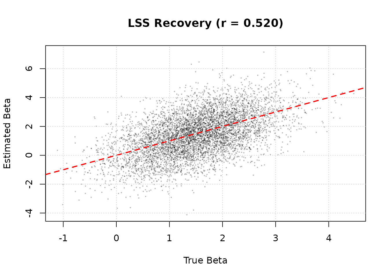

The fit is not perfect because the simulation adds substantial baseline structure and noise, but the recovered betas still track the ground truth in a way that is easy to diagnose numerically and visually.

Advanced: Parametric Modulators

event_model supports parametric modulators for trial-by-trial amplitude modulation. This example demonstrates the syntax but requires special setup.

# Trial data with reaction times
trials_rt <- data.frame(
  onset = c(10, 30, 50, 70, 90, 110),
  RT = c(0.5, 0.7, 0.6, 0.8, 0.5, 0.9),
  run = 1
)

# Center RT
trials_rt$RT_c <- scale(trials_rt$RT, center = TRUE, scale = FALSE)[, 1]

# Model: trial effects + RT modulation
emod_rt <- event_model(
  onset ~ trialwise() + hrf(RT_c),
  data = trials_rt,
  block = ~run,
  sampling_frame = sframe
)

# Note: This creates trial-wise regressors PLUS an RT amplitude modulator
# May require special handling in OASIS for proper separation

Troubleshooting

Error: “Y has X rows but sampling_frame expects Y scans”

Cause: Mismatch between data dimensions and sampling_frame specification.

Solution: Check that sum(blocklens) matches nrow(Y):

sframe_check <- sampling_frame(blocklens = c(150, 150), TR = 2)
sum(fmrihrf::blocklens(sframe_check))
#> [1] 300
nrow(Y)
#> [1] 300

Error: “event_model and baseline_model have different sampling_frames”

Cause: The two models were created with different sampling_frame objects.

Solution: Use the same sframe object for both:

sframe <- sampling_frame(blocklens = c(150, 150), TR = 2)

emod <- event_model(..., sampling_frame = sframe)
bmodel <- baseline_model(..., sframe = sframe)

Warning: “High collinearity detected”

Cause: Events are too close together or design is ill-conditioned.

Solution: Use ridge regularization:

beta <- lss_design(
  Y, emod, bmodel,
  oasis = list(ridge_mode = "fractional", ridge_x = 0.02)
)

Summary

The lss_design() function provides a modern, formula-based interface for LSS analysis that:

• Handles multi-run experiments correctly with run-relative onsets
• Provides structured baseline specification
• Supports multi-basis HRFs with automatic detection
• Validates design compatibility automatically
• Integrates with the fmridesign ecosystem

For simple designs or when you already have design matrices prepared, the traditional lss() interface remains fully supported and unchanged.

Further Reading

• vignette("fmrilss") - Traditional LSS interface
• vignette("oasis_method") - OASIS method details
• vignette("a_04_event_models", package = "fmridesign") - Event model tutorial
• vignette("a_03_baseline_model", package = "fmridesign") - Baseline model tutorial