Why fmrilss?
In rapid event-related fMRI, hemodynamic responses from consecutive trials overlap, making trial-by-trial beta estimates unstable. This is a problem for MVPA, RSA, and connectivity analyses that need reliable single-trial activation patterns.
Least Squares Separate (LSS; Mumford et al., 2012) solves this by fitting a separate GLM for each trial: one regressor for the trial of interest, one aggregating all other trials, plus nuisance regressors. This reduces collinearity and stabilizes estimates.
fmrilss provides optimized LSS implementations (R and
C++ with OpenMP), plus extensions for automatic HRF estimation, ridge
regularization, and the OASIS single-pass solver.
Quick example
Create a rapid event design
We’ll simulate 12 trials in a 150-TR run with jittered onsets, then convolve with a canonical HRF to build one design-matrix column per trial.
n_time <- 150
n_trials <- 12
n_vox <- 25
sframe <- sampling_frame(blocklens = n_time, TR = 1)

base <- round(seq(10, n_time - 24, length.out = n_trials))
onsets <- sort(pmax(10, pmin(base + sample(-3:3, n_trials, TRUE), n_time - 24)))
rset <- regressor_set(onsets, factor(seq_along(onsets)),
                      hrf = HRF_SPMG1, duration = 0, span = 24, summate = FALSE)
X <- evaluate(rset, grid = samples(sframe, global = TRUE),
              precision = 0.1, method = "conv")
X is a 150 x 12 matrix — one column per trial, each
containing the HRF-convolved impulse.
LSS vs standard GLM
The traditional approach (“Least Squares All”, LSA) estimates all trials in one model. Let’s compare:
beta_lsa <- lsa(Y, X, Z = Z, Nuisance = Nuisance)
comparison_summary <- data.frame(
  Method = c("LSS", "LSA"),
  CorrelationToTruth = c(
    cor(as.vector(beta_full), as.vector(true_betas)),
    cor(as.vector(beta_lsa), as.vector(true_betas))
  ),
  MeanTrialVariance = c(
    mean(apply(beta_full, 2, var)),
    mean(apply(beta_lsa, 2, var))
  )
)
comparison_summary
#>   Method CorrelationToTruth MeanTrialVariance
#> 1    LSS          0.9602123          1.675530
#> 2    LSA          0.8996540          2.163055
In this simulation, LSS is both less variable and closer to the known trial effects. A scatter plot shows how the two estimators relate to each other:
plot(as.vector(beta_lsa), as.vector(beta_full),
     pch = 19, col = adjustcolor("steelblue", 0.3), cex = 0.6,
     xlab = "LSA beta", ylab = "LSS beta",
     main = "Trial-wise betas: LSS vs LSA")
abline(0, 1, lty = 2, col = "gray40")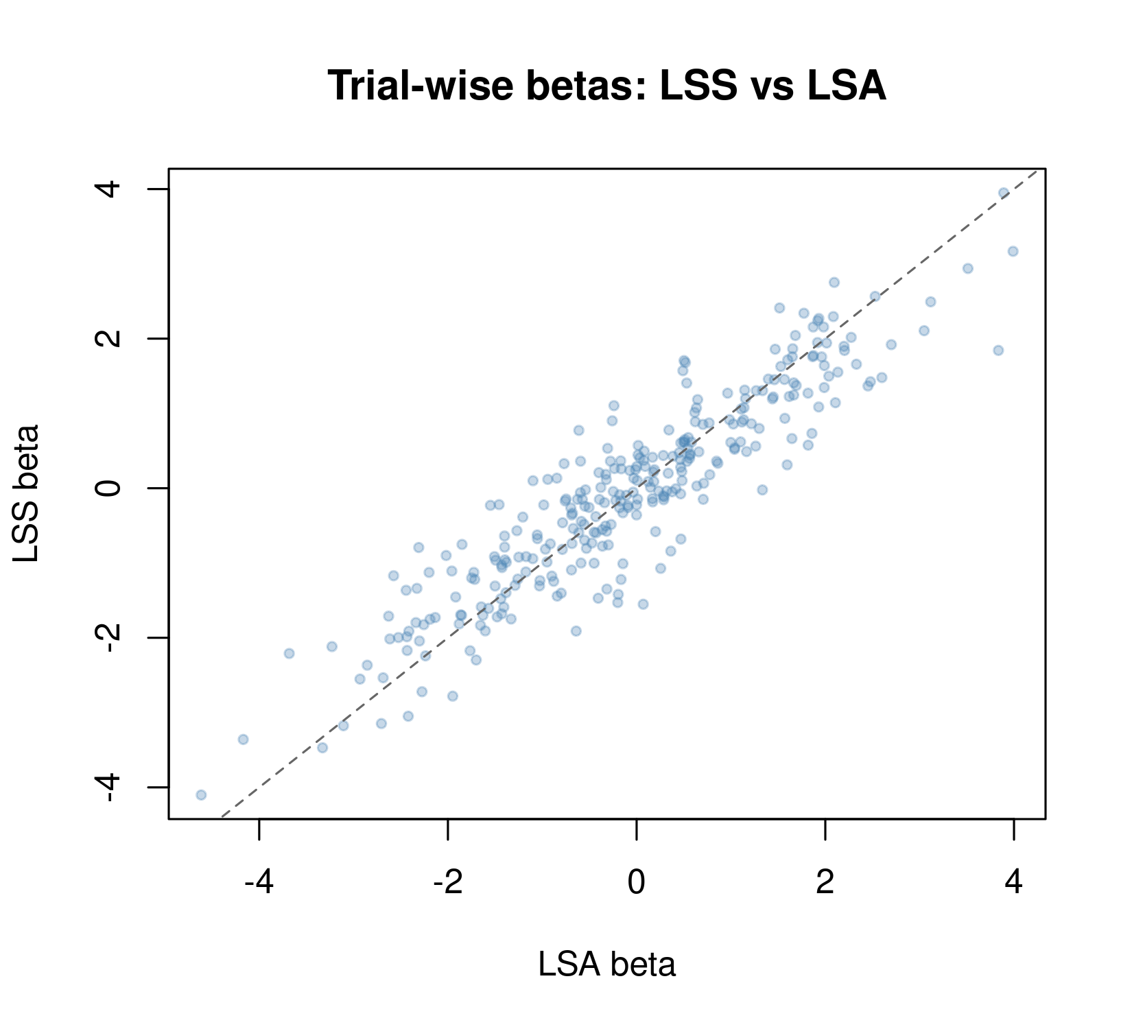
Prewhitening
fMRI time series have temporal autocorrelation. Pass a
prewhiten list to correct for it:
Automatic AR order selection:
beta_auto <- lss(Y, X, Z = Z, Nuisance = Nuisance,
                 prewhiten = list(method = "ar", p = "auto", p_max = 4))
See ?lss for additional pooling strategies
("voxel", "run", "parcel") and
ARMA models.
Computational backends
The default backend ("r_optimized") is fast and
readable. For large datasets, switch to the parallelized C++ engine:
beta_cpp <- lss(Y, X, Z = Z, Nuisance = Nuisance, method = "cpp_optimized")
all.equal(beta_full, beta_cpp, tolerance = 1e-8)
#> [1] TRUE
Available methods: "naive", "r_vectorized",
"r_optimized" (default), "cpp_optimized",
"oasis".
OASIS: single-pass LSS with extras
OASIS can build the design matrix from event specifications, add ridge regularization, and fit multi-basis HRFs — all in one call:
beta_oasis <- lss(
  Y, X = NULL, method = "oasis",
  oasis = list(
    design_spec = list(
      sframe = sframe,
      cond = list(onsets = onsets, hrf = HRF_SPMG1, span = 24)
    )
  )
)
dim(beta_oasis)
#> [1] 12 25
Setting X = NULL lets OASIS construct the design
internally from design_spec. Fractional ridge
regularization (5%) is applied by default to stabilize overlapping
designs. See vignette("oasis_method") for ridge tuning,
multi-basis HRFs, standard errors, and diagnostics.
Nuisance pre-projection
If you plan to re-run LSS with different settings, it can be faster to project out nuisance once up front:
Q <- project_confounds(Nuisance)
beta_pre <- lss(Q %*% Y, Q %*% X, Z = Z, method = "r_optimized")
This is useful when sweeping over hyperparameters (e.g., ridge values) without re-projecting nuisance regressors each time.
Next steps
-
vignette("oasis_method")— OASIS solver with ridge, multi-basis HRFs, and standard errors -
vignette("voxel-wise-hrf")— per-voxel HRF estimation before LSS -
vignette("sbhm")— library-constrained voxel-specific HRFs -
vignette("lss_with_fmridesign")— formula-based design interface for multi-run experiments