Introduction: Modeling Task Effects
An event model describes the expected BOLD signal changes related to experimental events (stimuli, conditions, responses, etc.). It forms the core of the task-related component of an fMRI General Linear Model (GLM).
fmridesign primarily uses the event_model()
function to create these models. It takes experimental design
information (event onsets, conditions, durations) and combines it with
Hemodynamic Response Function (HRF) specifications to generate the task
regressors.
This vignette focuses on the common formula-based interface for
event_model(). There’s also a list-based interface
(event_model.list) and a more programmatic
create_event_model() function for advanced use cases.
Quick HRF Primer
The hemodynamic response function (HRF) maps brief neural events to
predicted BOLD signal changes via convolution. In practice,
event_model() builds task regressors by convolving an event
train with a chosen HRF or with a set of HRF basis functions.
An HRF can be a single “canonical” shape (e.g., SPMG1) or a multi-basis set that allows the response shape to vary (e.g., SPMG2/3, tent/FIR, B‑splines). Multi-basis models produce multiple columns per condition, one for each basis function. Designs can use stick functions (zero duration) or boxcars (non‑zero duration) before convolution—choose this based on your experimental timing.
HRF definitions and generators live in the fmrihrf
package. See fmrihrf::gen_hrf() and the built‑in HRFs such
as fmrihrf::HRF_SPMG1, fmrihrf::HRF_SPMG2,
fmrihrf::HRF_SPMG3, fmrihrf::HRF_GAMMA,
fmrihrf::HRF_GAUSSIAN, and
fmrihrf::HRF_BSPLINE for details.
Timing and Sampling
The sampling_frame(TR, blocklens) defines the time grid
for your design (one row per scan, grouped by runs). Regressors are
generated on this grid. When events have non‑zero duration, the
convolution uses an internal time step to accurately approximate the
overlap of events and the HRF; fmrihrf handles
interpolation/upsampling under the hood so you don’t need to micromanage
it for typical use cases.
A Simple Single-Factor Design (Single Run)
Consider a basic design with four stimulus types (face, scene, tool, object), each presented 4 times for 2s, separated by a variable ISI (4-7s). The total scan duration is 70 TRs (TR=2s).
TR <- 2
cond <- c("face", "scene", "tool", "object")
NSTIM <- length(cond) * 4

# Construct the design table
set.seed(123) # for reproducibility
simple_design <- data.frame(
  stim = factor(sample(rep(cond, 4))),
  ISI = sample(10:20, NSTIM, replace = TRUE),  # Increased ISI range for better spacing
  run = rep(1, NSTIM),
  trial = factor(1:NSTIM)
)

# Calculate onsets (cumulative sum of duration (2s) + ISI)
simple_design$onset <- cumsum(c(0, simple_design$ISI[-NSTIM] + 2))

# Define the sampling frame (temporal structure of the scan)
sframe_single_run <- sampling_frame(blocklens = 140, TR = TR)

head(simple_design)
#>     stim ISI run trial onset
#> 1   tool  12   1     1     0
#> 2 object  20   1     2    14
#> 3   tool  18   1     3    36
#> 4  scene  18   1     4    56
#> 5  scene  18   1     5    76
#> 6  scene  12   1     6    96
Now, we create the event_model. The formula
onset ~ hrf(stim) specifies that:
-
onsetis the column insimple_designcontaining event start times. -
hrf(stim)defines a term where thestimfactor levels determine the conditions. Each level will be convolved with the default HRF (HRF_SPMG1).
The block = ~ run argument links events to scanning runs
(here, just one run).
emodel_simple <- event_model(onset ~ hrf(stim),
                             data = simple_design,
                             block = ~ run,
                             sampling_frame = sframe_single_run)

# Print the model summary
print(emodel_simple)
Visualizing the Event Model
We can plot the generated regressors using plot() (which
uses ggplot2) or plotly() for an interactive
version.
# Static plot (ggplot2)
plot(emodel_simple)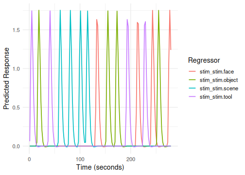
# Interactive plot via plotly (skipped in non-interactive builds)
if (interactive()) {
  plotly::ggplotly(plot(emodel_simple))
}
The plot shows the predicted BOLD timecourse for each condition
(stim level) convolved with the default HRF.
Design with Multiple Runs
Let’s extend the design to two runs.
# Construct a design table with two runs
design_list <- lapply(1:2, function(run_idx) {
  df <- data.frame(
    stim = factor(sample(rep(cond, 4))),
    ISI = sample(10:20, NSTIM, replace = TRUE),  # Increased ISI range for better spacing
    run = rep(run_idx, NSTIM)
  )
  df$onset <- cumsum(c(0, df$ISI[-NSTIM] + 2))
  df
})
design_multi_run <- bind_rows(design_list)

# Sampling frame for two runs of 140s each
sframe_multi_run <- sampling_frame(blocklens = c(140, 140), TR = TR)

head(design_multi_run)
#>     stim ISI run onset
#> 1   face  14   1     0
#> 2 object  17   1    16
#> 3  scene  11   1    35
#> 4   face  10   1    48
#> 5   tool  18   1    60
#> 6   face  20   1    80
The event_model call remains the same, but now
block = ~ run correctly maps events to their respective
runs based on the run column and the
sampling_frame.
emodel_multi_run <- event_model(onset ~ hrf(stim),
                                data = design_multi_run,
                                block = ~ run,
                                sampling_frame = sframe_multi_run)

print(emodel_multi_run)
# Plot without faceting - the plot method will handle multiple blocks
plot(emodel_multi_run)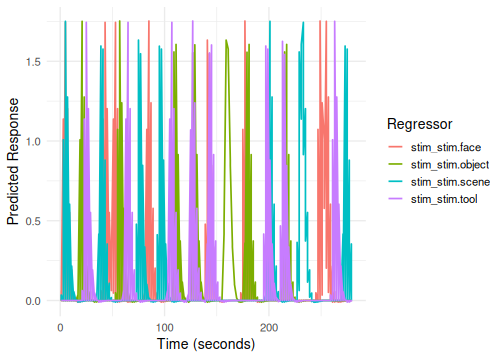
Two-Factor Design
Now consider a design crossing stimulus type (stim) with
task instruction (task: attend vs. ignore).
cond1 <- c("face", "scene", "tool", "object")
cond2 <- c("attend", "ignore")
comb <- expand.grid(stim = cond1, task = cond2)
NSTIM_TF <- nrow(comb) * 4 # 8 conditions * 4 reps per run

# Design for two runs
design_two_factor_list <- lapply(1:2, function(run_idx) {
  ind <- sample(rep(1:nrow(comb), length.out = NSTIM_TF))
  df <- data.frame(
    stim = factor(comb$stim[ind]),
    task = factor(comb$task[ind]),
    ISI = sample(6:15, NSTIM_TF, replace = TRUE),  # Increased ISI range for better spacing
    run = rep(run_idx, NSTIM_TF)
  )
  df$onset <- cumsum(c(0, df$ISI[-NSTIM_TF] + 2))
  df
})
design_two_factor <- bind_rows(design_two_factor_list)

# Sampling frame for two runs, potentially longer
sframe_two_factor <- sampling_frame(blocklens = c(200, 200), TR = TR)

head(design_two_factor)
#>     stim   task ISI run onset
#> 1  scene attend   8   1     0
#> 2  scene attend  14   1    10
#> 3 object attend  12   1    26
#> 4  scene attend  11   1    40
#> 5   tool ignore  15   1    53
#> 6  scene ignore  14   1    70
The formula onset ~ hrf(stim, task) automatically
creates regressors for the interaction of stim and
task. The term tag will default to
stim_task.
emodel_two_factor <- event_model(onset ~ hrf(stim, task),
                                 data = design_two_factor,
                                 block = ~ run,
                                 sampling_frame = sframe_two_factor)
print(emodel_two_factor)
# Column names will be like stim_task_stim.face_task.attend

# Plotting all interaction terms can be busy; consider plotly
plot(emodel_two_factor)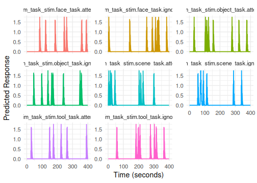
if (interactive()) {
  plotly::ggplotly(plot(emodel_two_factor))
}
Amplitude Modulation (Parametric Regressors)
We can model how a continuous variable (like reaction time, RT)
modulates the amplitude of the BOLD response. This is done by including
the modulating variable within the hrf() call.
# Use the simple single-run design and add a simulated RT column
simple_design$RT <- rnorm(nrow(simple_design), mean = 700, sd = 100)

# It's often recommended to center parametric modulators
simple_design$RT_centered <- scale(simple_design$RT, center = TRUE, scale = FALSE)[,1]
head(simple_design)
#>     stim ISI run trial onset       RT RT_centered
#> 1   tool  12   1     1     0 756.2990    34.12857
#> 2 object  20   1     2    14 662.7561   -59.41425
#> 3   tool  18   1     3    36 797.6973    75.52696
#> 4  scene  18   1     4    56 662.5419   -59.62846
#> 5  scene  18   1     5    76 805.2711    83.10077
#> 6  scene  12   1     6    96 595.0823  -127.08808
Here, hrf(stim) creates the main effect term (tag:
stim), and hrf(RT_centered) creates the
parametric modulator term (tag: RT_centered).
emodel_pmod <- event_model(onset ~ hrf(stim) + hrf(RT_centered),
                           data = simple_design,
                           block = ~ run,
                           sampling_frame = sframe_single_run)
print(emodel_pmod)
# Column names: stim_stim.face, ..., stim_stim.object, RT_centered_RT_centered

# Plot the RT parametric modulator term (using its term tag)
plot(emodel_pmod, term_name = "RT_centered") 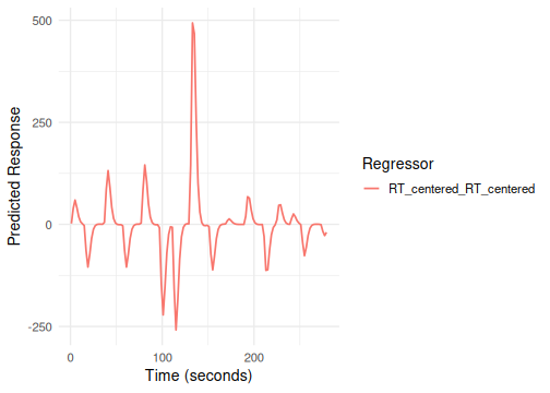
if (interactive()) {
  plotly::ggplotly(plot(emodel_pmod, term_name = "RT_centered"))
}
Interaction Between Factors and Amplitude Modulation
We can also model how a parametric modulator interacts with a factor.
For example, does RT modulate the response differently for faces
vs. scenes? The formula hrf(stim, RT_centered) creates
separate RT modulators for each level of stim.
Here, hrf(stim) is one term (tag: stim).
The interaction hrf(stim, RT_centered) is a second term
(tag: stim_RT_centered).
emodel_pmod_int <- event_model(onset ~ hrf(stim) + hrf(stim, RT_centered),
                               data = simple_design,
                               block = ~ run,
                               sampling_frame = sframe_single_run)
print(emodel_pmod_int)
# Columns: stim_stim.face, ..., stim_RT_centered_stim.face_RT_centered, ...

# Plot the interaction term (using its term tag)
plot(emodel_pmod_int, term_name = "stim_RT_centered")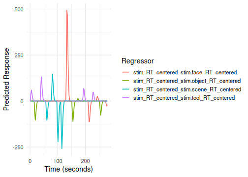
if (interactive()) {
  plotly::ggplotly(plot(emodel_pmod_int, term_name = "stim_RT_centered"))
}
Specifying Different HRFs
By default, hrf() uses the SPM canonical HRF
(HRF_SPMG1). You can specify a different HRF basis for any
term using the basis argument within the hrf()
call in the model formula.
Here are the main ways to specify the basis:
-
By Name (String): Use a recognized name for common HRFs:
-
"spmg1"(default),"spmg2","spmg3" -
"gaussian","gamma" -
"bspline"or"bs"(usenbasisto set number of splines) -
"tent"(usenbasisto set number of tent functions)
-
Using Pre-defined
HRFObjects: Pass an exportedHRFobject directly. Examples includeHRF_SPMG1,HRF_GAUSSIAN,HRF_SPMG2,HRF_SPMG3,HRF_BSPLINE,HRF_DAGUERRE,HRF_DAGUERRE_BASIS.Using Custom Functions
f(t): Provide your own function definition that accepts timetas the first argument.Using
gen_hrf()Results: Create a customized HRF usinggen_hrf(),hrf_blocked(),hrf_lagged(), etc., and pass the resultingHRFobject.
Discovering Available Options: You can easily
explore all available HRF types using the
list_available_hrfs() function:
# List basic information about available HRFs
list_available_hrfs()
#>        name      type nbasis_default is_alias
#> 1     spmg1    object              1    FALSE
#> 2     spmg2    object              2    FALSE
#> 3     spmg3    object              3    FALSE
#> 4     gamma    object              1    FALSE
#> 5  gaussian    object              1    FALSE
#> 6   bspline generator              5    FALSE
#> 7      tent generator              5    FALSE
#> 8   fourier generator              5    FALSE
#> 9  daguerre generator              3    FALSE
#> 10      fir generator             12    FALSE
#> 11      lwu generator       variable    FALSE
#> 12      gam    object              1    FALSE
#> 13       bs generator              5     TRUE

# Get detailed descriptions
list_available_hrfs(details = TRUE)
#>        name      type nbasis_default is_alias                description
#> 1     spmg1    object              1    FALSE        spmg1 HRF (object)
#> 2     spmg2    object              2    FALSE        spmg2 HRF (object)
#> 3     spmg3    object              3    FALSE        spmg3 HRF (object)
#> 4     gamma    object              1    FALSE        gamma HRF (object)
#> 5  gaussian    object              1    FALSE     gaussian HRF (object)
#> 6   bspline generator              5    FALSE   bspline HRF (generator)
#> 7      tent generator              5    FALSE      tent HRF (generator)
#> 8   fourier generator              5    FALSE   fourier HRF (generator)
#> 9  daguerre generator              3    FALSE  daguerre HRF (generator)
#> 10      fir generator             12    FALSE       fir HRF (generator)
#> 11      lwu generator       variable    FALSE       lwu HRF (generator)
#> 12      gam    object              1    FALSE          gam HRF (object)
#> 13       bs generator              5     TRUE bs HRF (generator) (alias)
For more details and examples of different HRF types, refer to the
documentation for hrf() and the HRF-related vignettes in
the fmrihrf package.
Here are a few examples within the event_model
context:
# Example 1: Using basis name string "gaussian"
# Term tags: "stim", "RT_centered"
emodel_diff_hrf <- event_model(onset ~ hrf(stim, basis="spmg1") + hrf(RT_centered, basis="gaussian"),
                               data = simple_design,
                               block = ~ run,
                               sampling_frame = sframe_single_run)
print(emodel_diff_hrf)
plot(emodel_diff_hrf, term_name = "RT_centered") # Plot the Gaussian RT regressor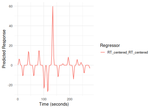
# Example 2: Using a pre-defined HRF object (SPMG3)
# Term tag: "stim"
emodel_spmg3 <- event_model(onset ~ hrf(stim, basis=HRF_SPMG3),
                            data = simple_design,
                            block = ~ run,
                            sampling_frame = sframe_single_run)
print(emodel_spmg3) # Note nbasis=3 for the hrf
# Columns: stim_stim.face_b01, stim_stim.face_b02, ...
plot(emodel_spmg3, term_name = "stim") # Plotting shows the 3 basis functions for one condition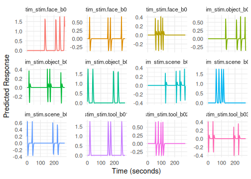
if (interactive()) {
  plotly::ggplotly(plot(emodel_spmg3)) # Better for exploring many conditions interactively
}

# Example 3: Using a custom function (simple linear ramp)
# Term tag: "stim"
linear_ramp_hrf <- function(t) { ifelse(t > 0 & t < 10, t/10, 0) }
emodel_custom_hrf <- event_model(onset ~ hrf(stim, basis=linear_ramp_hrf),
                                 data = simple_design,
                                 block = ~ run,
                                 sampling_frame = sframe_single_run)
print(emodel_custom_hrf)
plot(emodel_custom_hrf, term_name = "stim")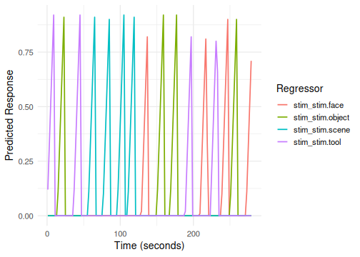
# Example 4: Using gen_hrf() to create a lagged Gaussian
# Term tag: "stim"
lagged_gauss <- gen_hrf(hrf_gaussian, lag = 2, name = "Lagged Gaussian")
emodel_gen_hrf <- event_model(onset ~ hrf(stim, basis = lagged_gauss),
                              data = simple_design,
                              block = ~ run,
                              sampling_frame = sframe_single_run)
print(emodel_gen_hrf)
plot(emodel_gen_hrf, term_name = "stim")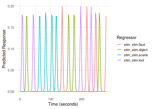
Per-Onset HRF Specification with hrf_fun
For advanced use cases where different events require different HRF
shapes, you can use the hrf_fun parameter. This accepts a
generator function that receives event data and returns a list of HRF
objects (one per onset). The generator is called after any
subsetting, so it only sees the events that will actually be
modeled.
# Generator function that assigns different HRFs based on condition
cond_hrf_gen <- function(event_data) {
  lapply(seq_len(nrow(event_data)), function(i) {
    if (event_data$stim[i] == "face") {
      HRF_SPMG1
    } else {
      HRF_GAMMA
    }
  })
}

emodel_per_onset <- event_model(
  onset ~ hrf(stim, hrf_fun = cond_hrf_gen),
  data = simple_design,
  block = ~ run,
  sampling_frame = sframe_single_run
)
print(emodel_per_onset)
The hrf_fun generator receives a data frame containing
onset, duration, blockid, and any
term variables. This enables use cases like:
-
Duration-based HRFs: Use
boxcar_hrf_gen()to create boxcar HRFs based on event duration -
Weighted sub-event HRFs: Use
weighted_hrf_gen()for events with sub-onset timing -
Formula syntax: Reference a column containing HRF
objects directly with
hrf_fun = ~my_hrf_column
# Create a design with varying event durations
boxcar_design <- data.frame(
  onset = c(0, 20, 45, 70),
  stim = factor(c("A", "B", "A", "B")),
  duration = c(2, 4, 3, 5),  # Varying durations
  run = 1
)

emodel_boxcar <- event_model(
  onset ~ hrf(stim, hrf_fun = boxcar_hrf_gen()),
  data = boxcar_design,
  durations = boxcar_design$duration,
  block = ~ run,
  sampling_frame = sframe_single_run
)
print(emodel_boxcar)
Advanced: Parametric Modulator with FIR HRF and Windowed F-contrast
Sometimes a parametric modulator is modeled with a multi‑basis HRF (e.g., FIR) to allow more flexible timing. In that case, the modulator produces multiple columns (one per basis bin). You can form an omnibus F‑test across a window of bins (e.g., around the expected peak) or across all bins.
# Toy design with a continuous RT modulator
set.seed(42)
n <- 60
des_pm <- data.frame(
  onset = sort(runif(n, 0, 260)),
  RT    = scale(runif(n, 0.4, 0.9))[,1],
  run   = 1
)
sframe_pm <- sampling_frame(blocklens = 140, TR = 2)

# Model RT with an FIR basis (10 bins)
emod_rt_fir <- event_model(
  onset ~ hrf(RT, basis = "fir", nbasis = 10),
  data = des_pm, block = ~ run, sampling_frame = sframe_pm
)

# Identify the RT columns in the full design matrix
dm <- design_matrix(emod_rt_fir)
idx <- term_indices(dm)    # maps term tags -> column indices
rt_cols <- idx[["RT"]]     # columns for the RT FIR term (b01..b10)
colnames(dm)[rt_cols][1:5]
#> [1] "RT_RT_b01" "RT_RT_b02" "RT_RT_b03" "RT_RT_b04" "RT_RT_b05"

# Build a windowed F-contrast over FIR bins 3:5 (peak region example)
window <- 3:5
win_cols <- rt_cols[window]
C_F <- matrix(0, nrow = ncol(dm), ncol = length(win_cols))
for (j in seq_along(win_cols)) C_F[win_cols[j], j] <- 1
colnames(C_F) <- paste0("RT_b", sprintf("%02d", window))

# Validate (treat `dm` as X); this reports an F-type contrast because C has multiple columns
validate_contrasts(dm, weights = C_F)
#>         name type estimable sum_to_zero orthogonal_to_intercept full_rank
#> 1 contrast#1    F      TRUE       FALSE                    TRUE      TRUE
#> 2 contrast#2    F      TRUE       FALSE                    TRUE      TRUE
#> 3 contrast#3    F      TRUE       FALSE                    TRUE      TRUE
#>   nonzero_weights
#> 1               1
#> 2               1
#> 3               1

# If you instead want a single t-contrast averaging the window, use 1/|window| weights
C_avg <- matrix(0, nrow = ncol(dm), ncol = 1)
C_avg[win_cols, 1] <- 1/length(win_cols)
colnames(C_avg) <- "RT_peak_avg"
validate_contrasts(dm, weights = C_avg)
#>       name type estimable sum_to_zero orthogonal_to_intercept full_rank
#> 1 contrast    t      TRUE       FALSE                    TRUE        NA
#>   nonzero_weights
#> 1               3
This pattern also works for other multi‑basis choices (e.g.,
SPMG2/3): build a contrast matrix that selects the columns for the
modulator’s basis functions and use validate_contrasts() to
confirm the contrast structure before fitting downstream.
Trialwise Models for Beta-Series Analysis
To model each trial individually (e.g., for beta-series correlation),
use trialwise() in the formula. This creates a separate
regressor for every single event specified by the onset
variable.
emodel_trialwise <- event_model(onset ~ trialwise(),
                                data = simple_design,
                                block = ~ run,
                                sampling_frame = sframe_single_run)
print(emodel_trialwise)
# Term tag: "trialwise"
# Columns: trialwise_trial.1, trialwise_trial.2, ...

# Plotting trialwise models can be very dense!
# It generates one condition per trial. Use label_mode/compactness controls.
plot(emodel_trialwise, label_mode = "none")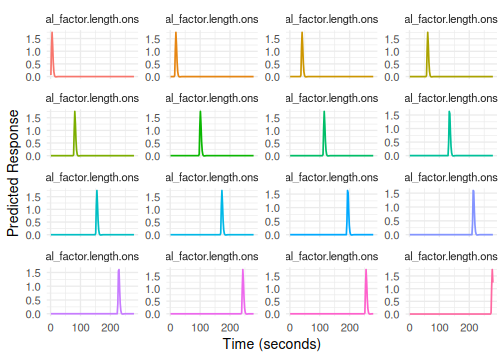
if (interactive()) {
  plotly::ggplotly(plot(emodel_trialwise, label_mode = "compact")) # Use plotly to explore interactively
}
Covariates (Non-convolved Regressors)
Sometimes you want to include scan-by-scan regressors that should not
be convolved with an HRF (e.g., motion, physiology). Use
covariate() within the formula. The covariate matrix must
have one row per scan (sum of blocklens).
Normally, one would add motion regressors to the
baseline_model but we use it as an illustrative
example.
# Create covariates aligned to the sampling frame
n_scans <- sum(blocklens(sframe_single_run))
motion <- data.frame(mx = rnorm(n_scans), my = rnorm(n_scans))

# Build a model with both convolved events and non-convolved covariates
emodel_cov <- event_model(onset ~ hrf(stim) + covariate(mx, my, data = motion, id = "motion"),
                          data = simple_design,
                          block = ~ run,
                          sampling_frame = sframe_single_run)
print(emodel_cov)

# Inspect columns; motion terms are added as-is
head(colnames(design_matrix(emodel_cov)))
#> [1] "stim_stim.face"   "stim_stim.object" "stim_stim.scene"  "stim_stim.tool"
#> [5] "mx"               "my"
Note: If the covariate rows do not match the number of scans, construction will error with a helpful message.
Accessing Model Components
Once an event_model is created, you can extract its
components:
# List the terms in the model (names are now term tags)
terms_list <- terms(emodel_pmod_int)
print(names(terms_list))
#> [1] "stim"             "stim_RT_centered"
# Expected: "stim", "stim_RT_centered"

# Get all condition names (full column names)
conds <- conditions(emodel_pmod_int)
# Example: stim_stim.face, stim_stim.scene, ...,
#          stim_RT_centered_stim.face_RT_centered, ...
cat("\nFirst 6 column names:", head(colnames(design_matrix(emodel_pmod_int)), 6), "...\n")
#>
#> First 6 column names: stim_stim.face stim_stim.object stim_stim.scene stim_stim.tool stim_RT_centered_stim.face_RT_centered stim_RT_centered_stim.object_RT_centered ...

# Extract the full design matrix
dmat_events <- design_matrix(emodel_pmod_int)
cat("\nEvent design matrix dimensions:", dim(dmat_events), "\n")
#>
#> Event design matrix dimensions: 140 8
head(dmat_events[, 1:6])
#> # A tibble: 6 × 6
#>   stim_stim.face stim_stim.object stim_stim.scene stim_stim.tool
#>            <dbl>            <dbl>           <dbl>          <dbl>
#> 1              0                0               0     0.06243065
#> 2              0                0               0     1.137517
#> 3              0                0               0     1.743962
#> 4              0                0               0     1.202648
#> 5              0                0               0     0.5518543
#> 6              0                0               0     0.1917313
#> # ℹ 2 more variables: stim_RT_centered_stim.face_RT_centered <dbl>,
#> #   stim_RT_centered_stim.object_RT_centered <dbl>

# Contrast weights and F-contrasts can also be extracted (see contrasts vignette)
contrast_weights(emodel_pmod_int)
#> list()
Fcontrasts(emodel_pmod_int)
#> $`stim#stim`
#>                                          c1 c2 c3
#> stim_stim.face                            1  0  0
#> stim_stim.object                          0  1  0
#> stim_stim.scene                           0  0  1
#> stim_stim.tool                           -1 -1 -1
#> stim_RT_centered_stim.face_RT_centered    0  0  0
#> stim_RT_centered_stim.object_RT_centered  0  0  0
#> stim_RT_centered_stim.scene_RT_centered   0  0  0
#> stim_RT_centered_stim.tool_RT_centered    0  0  0
#> attr(,"term_indices")
#> [1] 1 2 3 4
#>
#> $`stim_RT_centered#stim`
#>                                          c1 c2 c3
#> stim_stim.face                            0  0  0
#> stim_stim.object                          0  0  0
#> stim_stim.scene                           0  0  0
#> stim_stim.tool                            0  0  0
#> stim_RT_centered_stim.face_RT_centered    1  0  0
#> stim_RT_centered_stim.object_RT_centered  0  1  0
#> stim_RT_centered_stim.scene_RT_centered   0  0  1
#> stim_RT_centered_stim.tool_RT_centered   -1 -1 -1
#> attr(,"term_indices")
#> [1] 5 6 7 8
Visualizing the Design Matrix and Correlations
Two functions help visualize the structure of the event design matrix:
-
design_map: Shows the matrix values as a heatmap. -
correlation_map: Shows the correlation between regressors.
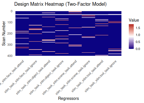
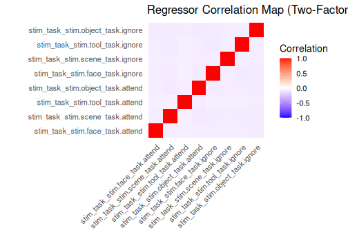
Note: Axis labels are hidden above to keep the heatmaps legible with
many regressors. When exploring smaller models interactively, set
rotate_x_text = TRUE (and remove the
theme(...) line) to show labels.
This event_model represents the task-related part of the
fMRI model. In practice, you will combine it with a
baseline_model (drift/intercepts/nuisance) to form a full
design matrix; downstream GLM fitting happens in analysis packages
(e.g., fmrireg).
Contrasts Quickstart
You can attach contrasts directly to hrf() terms. Here
are two common patterns.
# Pairwise contrast between two stimulus levels
con_face_vs_scene <- pair_contrast(~ stim == "face", ~ stim == "scene", name = "face_vs_scene")

emodel_con <- event_model(onset ~ hrf(stim, contrasts = contrast_set(con_face_vs_scene)),
                          data = simple_design,
                          block = ~ run,
                          sampling_frame = sframe_single_run)

# List available contrast specs and weights
contr_specs <- contrasts(emodel_con)
cw <- contrast_weights(emodel_con)
names(cw)
#> [1] "stim#face_vs_scene"

# One-way contrast (main effect over levels of a factor)
con_main_stim <- oneway_contrast(~ stim, name = "main_stim")
emodel_con2 <- event_model(onset ~ hrf(stim, contrasts = contrast_set(con_main_stim)),
                           data = simple_design,
                           block = ~ run,
                           sampling_frame = sframe_single_run)

fcons <- Fcontrasts(emodel_con2)
names(fcons)
#> [1] "stim#stim"
Combining Event and Baseline Designs
To build a full design matrix, bind the event regressors with the baseline regressors.
# Baseline model for the same sampling frame
bmodel <- baseline_model(basis = "poly", degree = 5, sframe = sframe_two_factor)

# Combine columns (order can matter downstream; keep consistent)
DM_full <- dplyr::bind_cols(design_matrix(emodel_two_factor), design_matrix(bmodel))
dim(DM_full)
#> [1] 400  20
colnames(DM_full)[1:8]
#> [1] "stim_task_stim.face_task.attend"   "stim_task_stim.scene_task.attend"
#> [3] "stim_task_stim.tool_task.attend"   "stim_task_stim.object_task.attend"
#> [5] "stim_task_stim.face_task.ignore"   "stim_task_stim.scene_task.ignore"
#> [7] "stim_task_stim.tool_task.ignore"   "stim_task_stim.object_task.ignore"
Downstream GLM fitting occurs in analysis packages (e.g., fmrireg), but fmridesign provides consistent, inspectable design matrices you can feed into those tools.