GLMsingle in fmrilss: library HRFs, GLMdenoise and fractional ridge

What GLMsingle estimates

GLMsingle (Prince et al., 2022) estimates one response amplitude per trial and voxel. Use glmsingle() when you want to select an HRF from a library, estimate shared noise regressors, and choose ridge shrinkage from repeated conditions across runs. The procedure builds on a single-trial general linear model (GLM):

1. Select an HRF per voxel (type B). Choose the best-fitting shape from a library of 20 haemodynamic response functions (HRFs).
2. Add GLMdenoise regressors (type C). Identify a pool of voxels with weak task fit, remove polynomial trends from their time series, and use principal components (PCs) of the normalized residuals as nuisance regressors. Cross-validation selects the number of PCs.
3. Apply fractional ridge regression (type D). Cross-validation selects shrinkage separately for each voxel. By default, the ridge estimates are then rescaled and offset to best match the unregularised estimates.

An initial ON-OFF model (type A) uses one regressor for all trials and helps define the noise pool. Both default cross-validations compare trial betas for the same condition in different runs. Without those repeats, their data-driven choices are unavailable; the function warns and disables the stages that require them.

The implementation solves each run separately and reuses matrix products to score candidate models. The final sections describe the differences from the reference implementation and how numerical agreement is tested.

A simulated experiment

The simulation has four runs of 110 time points, sampled every second. Each run contains trials from eight conditions, with every condition repeated across runs. Voxels differ in HRF shape and share slow structured noise. Eighty voxels respond to the task; the remaining forty provide a potential noise pool for GLMdenoise.

library(fmrilss)
set.seed(2024)
tr <- 1; stimdur <- 3
n_runs <- 4; n_time <- 110; n_vox <- 120; n_cond <- 8
lib <- glmsingle_hrf_library(stimdur, tr)
true_hrf <- sample(ncol(lib), n_vox, replace = TRUE)
responsive <- seq_len(n_vox) <= 80
cond_mean <- matrix(rnorm(n_cond * n_vox, 1.5, 1), n_cond)
load <- matrix(rnorm(3 * n_vox, 0, 1.5), 3)

design <- Y <- true_beta <- vector("list", n_runs)
for (r in seq_len(n_runs)) {
  onsets <- seq(3, n_time - 15, by = 4) + sample(0:1, 1)
  cond <- sample(rep_len(seq_len(n_cond), length(onsets)))
  D <- matrix(0, n_time, n_cond)
  D[cbind(onsets + 1, cond)] <- 1
  amp <- cond_mean[cond, ] + matrix(rnorm(length(onsets) * n_vox, 0, 0.5), length(onsets))
  amp[, !responsive] <- 0
  signal <- vapply(seq_len(n_vox), function(v) {
    s <- numeric(n_time); s[onsets + 1] <- amp[, v]
    stats::convolve(s, rev(lib[, true_hrf[v]]), type = "open")[seq_len(n_time)]
  }, numeric(n_time))
  latent <- apply(matrix(rnorm(3 * n_time), n_time), 2, cumsum) * 0.4
  noise <- matrix(rnorm(n_time * n_vox), n_time) + latent %*% load
  Y[[r]] <- 1000 * (1 + 0.01 * (signal + noise))
  design[[r]] <- D
  true_beta[[r]] <- amp
}
true_beta <- do.call(rbind, true_beta)  # trials x voxels, chronological

design contains one time-by-condition 0/1 matrix per run, with a 1 at each trial onset. Unlike the trial matrices passed to lss(), these are onset indicators, not HRF-convolved regressors.

You can also supply a data frame with run, onset (seconds, on the TR grid), and condition columns, or use glmsingle_design() with an fmridesign event model. For list-valued Y, ascending event run IDs correspond to the list order. For a single data matrix, supply scan-level runs; event IDs are matched to the runs in data order.

Fitting

fit <- glmsingle(Y, design, tr = tr, stimdur = stimdur, verbose = FALSE)
fit
#> <glmsingle_fit>
#>   4 runs, 96 trials, 8 conditions, 120 voxels
#>   models: A (ON-OFF), B (HRF library), C (GLMdenoise), D (fractional ridge) 
#>   noise PCs selected: 3
#>   median ridge fraction: 0.70
#>   elapsed: 0.5 s

The result contains typea, typeb, typec, and typed lists using GLMsingle’s field names. Types B–D contain trial-by-voxel betas, ordered by run and then by onset within each run. Betas are in percent signal change by default. coef(fit) extracts type D; pass "b" or "c" to extract an earlier stage.

dim(coef(fit))            # type D
#> [1]  96 120
fit$typed$pcnum           # number of GLMdenoise components
#> [1] 3

A ridge fraction of 1 means no shrinkage; smaller fractions request more shrinkage before the final rescaling. pcnum is the selected number of noise components, shared across voxels; FRACvalue contains one fraction per voxel.

What did cross-validation choose?

The left panel shows xvaltrend: the negative median cross-validation loss over the voxels used to choose the PC count. Higher is better; it measures agreement between betas for repeated conditions across runs, not time-series R^2. With the default pcstop = 1.05, the algorithm takes the first PC count whose improvement over zero PCs is at least 1 / 1.05 (about 95%) of the best improvement. The dashed line marks that threshold, and the red point marks the selected count.

The right panels show the selected ridge fractions separately for the two simulated voxel groups. These labels come from the generating model, not from GLMsingle’s estimated noise pool. Counts have a common scale; the groups contain 80 and 40 voxels, respectively.

pc_scores <- data.frame(
  PCs = seq_along(fit$typec$xvaltrend) - 1L,
  score = fit$typec$xvaltrend
)
pc_threshold <- pc_scores$score[1] +
  (max(pc_scores$score) - pc_scores$score[1]) / fit$settings$pcstop
ridge_choices <- data.frame(
  fraction = fit$typed$FRACvalue,
  group = ifelse(responsive, "Task-responsive\n(n = 80)", "No task response\n(n = 40)")
)

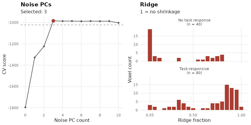
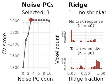
Cross-validation diagnostics from the same fit. Ridge fractions describe shrinkage before the default final rescaling and offset; they are not the final ratio of estimated to true amplitude.

Did the data-driven steps help?

Because the generating amplitudes are known, we can compare estimated and true betas in the responsive voxels. For each voxel, we correlate estimated and true amplitudes across all trials. This measures agreement in trial-to-trial variation, but does not measure amplitude bias or absolute estimation error. Correlation is undefined for the forty nonresponsive voxels, whose true amplitudes are all zero, so they are excluded here.

voxel_cor <- sapply(c("b", "c", "d"), function(stage) {
  B <- coef(fit, stage)
  vapply(which(responsive), function(v) {
    stats::cor(B[, v], true_beta[, v])
  }, numeric(1))
})
round(colMeans(voxel_cor), 3)
#>     b     c     d 
#> 0.334 0.601 0.660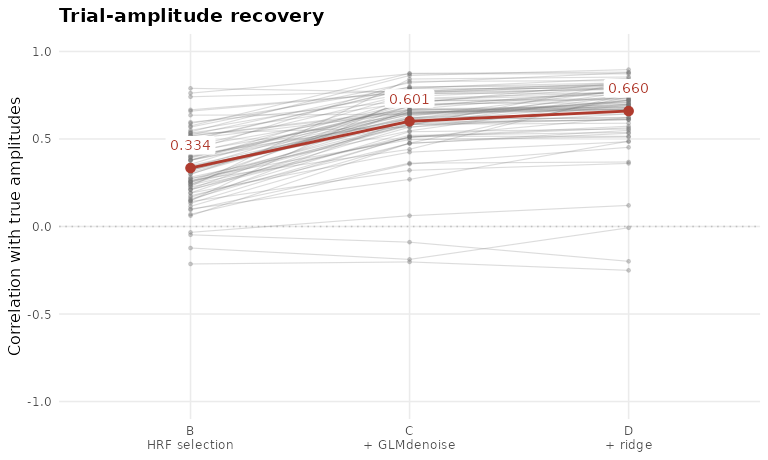

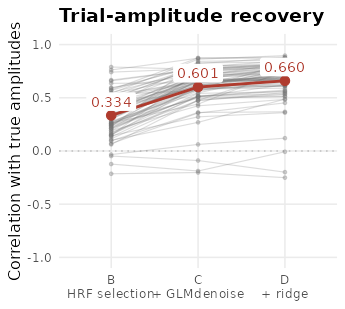
Each thin line follows one of the 80 responsive voxels; red points and labels show the mean at each stage. The spread and downward segments remain visible alongside the average improvement.

In this simulation, mean recovery improves from B to C and again from C to D. The voxel-level lines show why the mean alone is incomplete: 3 voxels have lower correlations after denoising, and 2 after ridge. A useful step on average need not help every voxel. This is one fixed simulated experiment, not a guarantee of improvement for another acquisition.

Which HRF shapes were recovered?

The library contains responses to a 3-second stimulus, sampled every 1 second and normalized to a peak of one. Its 20 shapes differ in their timing, width, and undershoot. The first panel shows the full library; the remaining panels compare the generating and selected shapes for voxels 1, 2, and 3, chosen by index before inspecting recovery.

example_voxels <- 1:3
data.frame(voxel = example_voxels,
           true_index = true_hrf[example_voxels],
           selected_index = fit$typeb$HRFindex[example_voxels])
#>   voxel true_index selected_index
#> 1     1          2              2
#> 2     2          5              8
#> 3     3         13             13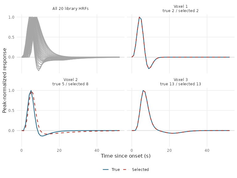

All curves use the same time and peak-normalized amplitude scales. Solid blue curves are the generating HRFs; dashed red curves are the selected library shapes. Coincident curves indicate an exact library match.

Nearby library indices do not necessarily imply equally small waveform differences, so the curves are more informative than index distance alone. These examples illustrate the selection step; the recovery plot above uses all responsive voxels.

Choices that differ from the reference implementation

Two defaults differ from the pinned Python reference (commit 1ab54a6):

Argument	fmrilss default	Option that follows the Python reference
extras_in_denoise	"always": retain user nuisance regressors, such as motion, in every GLMdenoise and ridge fit	"with_pcs": omit them when zero PCs are used, including from the cross-validation reference
zero_sd_cv	"zero": give zero cross-validation weight to voxels whose reference betas have zero variance	"python": reproduce the reference helper’s candidate-dependent treatment of zero variance

Two further options control singular designs and the ridge calculation. singular = "error" follows GLMsingle’s default; "pinv" instead returns a minimum-norm solution with a warning. frac_alpha = "fracridge" uses the reference grid interpolation to obtain ridge penalties; "exact" solves the fraction equation directly and is experimental.

The automatic ON-OFF R^2 threshold uses a deterministic Gaussian-mixture fit with a small variance floor, following the MATLAB approach; the Python mixture fit is unseeded. Pass brain_r2 and pc_r2_cutoff to set the thresholds explicitly. Empty or rank-zero noise pools use zero PCs; otherwise the maximum PC count is capped at the available rank across runs.

fmrilss computes in double precision, uses 1-based HRF indices, and applies want_percent_bold to all model types. The Python reference uses single precision and always scales types C and D to percent signal change.

full_glmbadness = TRUE fills the PC cross-validation diagnostic for every voxel. By default only the voxels that decide the number of PCs are evaluated, which gives identical estimates.

How agreement with GLMsingle is checked

The package tests compare glmsingle() with pinned Python GLMsingle on 11 simulated scenarios: default settings, extra regressors, two sessions with grouped folds, unequal run lengths, unrepeated conditions, rapid events, near-collinear regressors, an all-zero voxel, a single ridge fraction, and no HRF library. The tests require matching HRF choices and PC counts. Beta and ridge-fraction comparisons exclude cases classified as numerically unstable in the Python reference. Beta tolerances depend on the design’s condition number, accounting for the loss of precision in float32 normal equations; they do not impose a uniform 1e-6 bound.

Separate tests compare the computational stages in double precision with dense implementations of GLMsingle’s stacked calculations. Together, these checks test implementation agreement in the specified scenarios; they do not establish which estimator is best for a new acquisition.

Reference

Prince, J. S., Charest, I., Kurzawski, J. W., Pyles, J. A., Tarr, M. J., & Kay, K. N. (2022). Improving the accuracy of single-trial fMRI response estimates using GLMsingle. eLife, 11, e77599.