Multiset Manifold Alignment with mma_align

Overview

mma_align_multiple() aligns three or more domains by combining heat-kernel spectral embeddings, eigensignature-based eigenbasis registration, and an EM refinement step that supports both reference matching and joint consensus templates. The function exposes controls for histogram versus Wasserstein signatures, gating heuristics for repeated eigenvalues, and final Hungarian assignments when hard correspondences are needed.

This vignette follows the style of the other tutorials in the package: we build a multiset from the shared alignment_benchmark, run both reference and consensus modes, and inspect diagnostics returned by alignment_quality().

Setup

library(manifoldalign)
library(multidesign)
library(tibble)
library(dplyr)
library(ggplot2)

Preparing the Multiset Example

alignment_benchmark <- manifoldalign::alignment_benchmark
raw_domains <- alignment_benchmark$domains

multi_domains <- lapply(raw_domains, function(dom) {
  multidesign::multidesign(dom$x, dom$design)
})

multi_names <- names(multi_domains)
node_counts <- vapply(multi_domains, function(dom) nrow(dom$x), integer(1))

hd_multi <- multidesign::hyperdesign(multi_domains)

tibble(
  domain = multi_names,
  nodes = node_counts,
  features = vapply(multi_domains, function(dom) ncol(dom$x), integer(1))
)
#> # A tibble: 3 × 3
#>   domain  nodes features
#>   <chr>   <int>    <int>
#> 1 domain1    80        4
#> 2 domain2    80        4
#> 3 domain3    80        4

The latent classes shipped with the benchmark are used only for diagnostics.

table(multi_domains[[1]]$design$condition)
#> 
#> class_A class_B 
#>      40      40

Reference Mode Alignment

We first align every domain to domain1 with eigensignature gating, hypersphere normalisation, and a final Hungarian pass to extract hard correspondences.

set.seed(1)
mma_ref <- mma_align_multiple(
  hd_multi,
  ref_idx = 1,
  ncomp = 8,
  sigma = 0.7,
  embedding = "ctd",
  normalize = "hypersphere",
  match_to = "reference",
  signature_method = "hybrid",
  signature_gate_multiplicity = TRUE,
  signature_retry_if_weak = TRUE,
  final_assignment = "hungarian"
)

str(mma_ref, max.level = 1)
#> List of 15
#>  $ v              : num [1:12, 1:8] -44.57 -54.31 -42.32 -34.32 6.87 ...
#>  $ s              : num [1:240, 1:8] -0.736 -0.711 -0.936 -0.656 -0.74 ...
#>  $ sdev           : num [1:8] 0.515 0.511 0.245 0.337 0.305 ...
#>  $ preproc        : NULL
#>  $ block_indices  :List of 3
#>  $ rotations      :List of 3
#>  $ posteriors     :List of 3
#>  $ hist_align     :List of 3
#>  $ signature_align:List of 3
#>  $ ref_idx        : num 1
#>  $ embedding      : chr "ctd"
#>  $ normalize      : chr "hypersphere"
#>  $ K              : int 8
#>  $ assignment     :List of 3
#>  $ em_stats       :List of 3
#>  - attr(*, "class")= chr [1:2] "mma_align_multiple" "multiblock_biprojector"

quality_ref <- alignment_quality(mma_ref)

tibble::as_tibble(quality_ref$per_domain)
#> # A tibble: 3 × 9
#>   domain     n    mse mse_soft matched coverage mean_confidence converged
#>    <int> <int>  <dbl>    <dbl>   <int>    <dbl>           <dbl> <lgl>    
#> 1      1    80 NA     NA            NA       NA          NA     TRUE     
#> 2      2    80  0.265  0.0117       80        1           0.486 FALSE    
#> 3      3    80  0.196  0.00270      80        1           0.517 FALSE    
#> # ℹ 1 more variable: iterations <int>

tibble::as_tibble(quality_ref$global)
#> # A tibble: 1 × 6
#>   mse_weighted mse_soft_weighted     K ref_idx mean_confidence all_converged
#>          <dbl>             <dbl> <int>   <dbl>           <dbl> <lgl>        
#> 1        0.230           0.00481     8       1           0.501 FALSE

The per-domain diagnostics expose EM convergence, average eigensignature confidence, and MSE under both hard and soft correspondences. We can relate the assignments back to the hidden labels of the benchmark.

ref_conditions <- multi_domains[[1]]$design$condition

class_accuracy <- vapply(seq_along(multi_names)[-1], function(idx) {
  perm <- mma_ref$assignment[[idx]]
  keep <- which(!is.na(perm))
  if (!length(keep)) return(NA_real_)
  mean(ref_conditions[perm[keep]] == multi_domains[[idx]]$design$condition[keep])
}, numeric(1))

coverage <- quality_ref$per_domain$coverage[-1]

accuracy_tbl <- tibble(
  domain = multi_names[-1],
  class_accuracy = class_accuracy,
  hard_match_coverage = coverage
)

accuracy_tbl
#> # A tibble: 2 × 3
#>   domain  class_accuracy hard_match_coverage
#>   <chr>            <dbl>               <dbl>
#> 1 domain2          0.225                   1
#> 2 domain3          0.225                   1

The aligned embeddings combine all domains row-wise. Visual inspection of the first two components highlights the shared latent structure recovered by mma_align_multiple().

score_tbl <- as_tibble(as.matrix(mma_ref$s), .name_repair = "minimal")
colnames(score_tbl) <- paste0("comp", seq_len(ncol(score_tbl)))

score_tbl <- score_tbl %>%
  mutate(
    domain = rep(multi_names, times = node_counts),
    condition = unname(unlist(lapply(multi_domains, function(dom) dom$design$condition)))
  )

 ggplot(score_tbl, aes(x = comp1, y = comp2, colour = condition, shape = domain)) +
  geom_point(alpha = 0.85, size = 2) +
  labs(title = "Reference-mode MMA embeddings", x = "Component 1", y = "Component 2") +
  theme_minimal()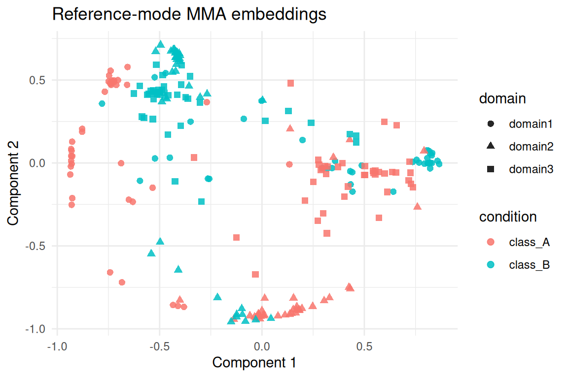

Scatter of MMA reference-mode embeddings across domains and latent classes

Consensus Template Mode

Consensus mode learns a shared orthogonal template while allowing uneven domain sizes. We down-sample domain3 to 60 nodes to illustrate the automatic choice of consensus centres (min by default).

set.seed(42)
consensus_domains <- raw_domains
keep_idx <- sort(sample(seq_len(nrow(consensus_domains[[3]]$x)), 60))
consensus_domains[[3]]$x <- consensus_domains[[3]]$x[keep_idx, , drop = FALSE]
consensus_domains[[3]]$design <- consensus_domains[[3]]$design[keep_idx, ]

multi_consensus <- lapply(consensus_domains, function(dom) {
  multidesign::multidesign(dom$x, dom$design)
})

consensus_names <- names(multi_consensus)
consensus_counts <- vapply(multi_consensus, function(dom) nrow(dom$x), integer(1))

hd_consensus <- multidesign::hyperdesign(multi_consensus)

tibble(
  domain = consensus_names,
  nodes = consensus_counts
)
#> # A tibble: 3 × 2
#>   domain  nodes
#>   <chr>   <int>
#> 1 domain1    80
#> 2 domain2    80
#> 3 domain3    60

set.seed(99)
mma_consensus <- mma_align_multiple(
  hd_consensus,
  ref_idx = 1,
  ncomp = 8,
  sigma = 0.7,
  embedding = "ctd",
  normalize = "hypersphere",
  match_to = "consensus",
  consensus_centers = "min",
  consensus_init = "ref",
  signature_method = "w2",
  eig_penalty = 0.01,
  signature_gate_multiplicity = TRUE,
  final_assignment = "hungarian",
  em_outlier = 0.05
)

list(
  consensus_centers = nrow(mma_consensus$consensus),
  em_iterations = mma_consensus$em_stats$iterations,
  converged = mma_consensus$em_stats$converged
)
#> $consensus_centers
#> [1] 60
#> 
#> $em_iterations
#> [1] 7
#> 
#> $converged
#> [1] TRUE

quality_consensus <- alignment_quality(mma_consensus)

tibble::as_tibble(quality_consensus$per_domain)
#> # A tibble: 3 × 9
#>   domain     n   mse    mse_soft matched coverage mean_confidence converged
#>    <int> <int> <dbl>       <dbl>   <int>    <dbl>           <dbl> <lgl>    
#> 1      1    80 0.254  0.00000859      60     0.75          NA     TRUE     
#> 2      2    80 0.241 NA               60     0.75           0.995 TRUE     
#> 3      3    60 0.259 NA               60     1              0.993 TRUE     
#> # ℹ 1 more variable: iterations <int>

tibble::as_tibble(quality_consensus$global)
#> # A tibble: 1 × 6
#>   mse_weighted mse_soft_weighted     K ref_idx mean_confidence all_converged
#>          <dbl>             <dbl> <int>   <dbl>           <dbl> <lgl>        
#> 1        0.251        0.00000312     8       1           0.994 TRUE

The consensus template captures the shared geometry in a compact basis. Each domain’s embeddings sit close to the learned centres even though domain3 has fewer nodes.

consensus_scores <- as_tibble(as.matrix(mma_consensus$s), .name_repair = "minimal")
colnames(consensus_scores) <- paste0("comp", seq_len(ncol(consensus_scores)))

consensus_scores <- consensus_scores %>%
  mutate(
    domain = rep(consensus_names, times = consensus_counts),
    condition = unname(unlist(lapply(multi_consensus, function(dom) dom$design$condition)))
  )

centers_tbl <- tibble(
  comp1 = mma_consensus$consensus[, 1],
  comp2 = mma_consensus$consensus[, 2],
  domain = "consensus",
  condition = factor("template")
)

plot_tbl <- bind_rows(
  mutate(consensus_scores, marker = "nodes"),
  mutate(centers_tbl, marker = "centres")
)

 ggplot(plot_tbl, aes(x = comp1, y = comp2, colour = condition, shape = marker)) +
  geom_point(alpha = 0.85, size = 2) +
  labs(title = "Consensus-mode MMA embeddings", x = "Component 1", y = "Component 2") +
  theme_minimal()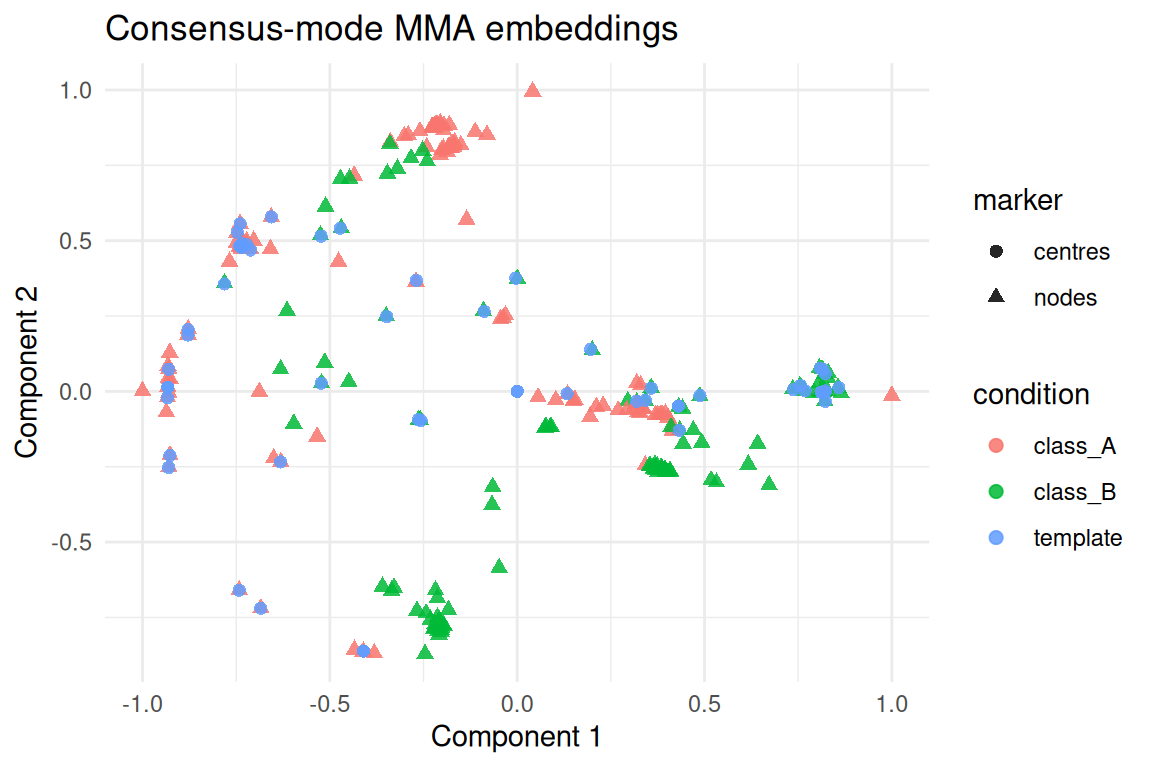

Consensus-mode MMA embeddings with domain points and learned centres

Consensus assignments point each domain back to indices of the template. The coverage column in alignment_quality() indicates how many nodes land on a unique centre; increasing em_outlier or switching final_assignment to "argmax" can trade precision for recall when outliers are expected.

Summary