Generalized PCA Alignment with gpca_align

Overview

gpca_align() implements Generalized PCA alignment. It constructs a coupled metric across domains and then solves a generalized PCA problem to obtain a shared latent embedding. The helper gpca_align_control() exposes safeguards for graph sparsification, label balancing and dense-matrix memory limits, making it practical on real data.

This vignette walks through a minimal pipeline:

1. Load a reusable hyperdesign dataset with three related domains.
2. Run gpca_align() and inspect the aligned scores.
3. Tune graph sparsity and balancing with gpca_align_control().

The code below only relies on public package APIs, so you can copy–paste it when exploring your own data.

Setup

library(manifoldalign)
library(multidesign)
library(multivarious)
library(tibble)
library(dplyr)
library(ggplot2)
library(purrr)

Constructing a Hyperdesign

We reuse the packaged benchmark dataset so every alignment vignette operates on identical inputs. It contains three domains with two latent classes and moderate domain-specific transformations.

alignment_benchmark <- manifoldalign::alignment_benchmark
domain_list <- lapply(alignment_benchmark$domains, function(dom) {
  multidesign(dom$x, dom$design)
})
hd <- hyperdesign(domain_list)
labels <- alignment_benchmark$labels
domain_names <- names(domain_list)
domain_sizes <- vapply(domain_list, function(dom) nrow(dom$x), integer(1))

When data is a hyperdesign, call gpca_align() and supply the label column name via the y argument.

base_preproc <- replicate(length(domain_names), multivarious::pass(), simplify = FALSE)

gpca_fit <- gpca_align(
  hd,
  y = condition,
  ncomp = 2,
  u = 0.6,           # balance within/between alignment
  lambda = 1e-2,     # light ridge regularisation
  preproc = base_preproc
)

str(gpca_fit, max.level = 1)
#> List of 6
#>  $ v            : num [1:12, 1:2] -0.342 -0.361 -0.294 -0.246 -0.306 ...
#>   ..- attr(*, "dimnames")=List of 2
#>  $ preproc      :List of 2
#>   ..- attr(*, "class")= chr [1:2] "concat_pre_processor" "pre_processor"
#>  $ s            : num [1:240, 1:2] -0.112 -0.153 -0.161 -0.201 -0.148 ...
#>   ..- attr(*, "dimnames")=List of 2
#>  $ sdev         : num [1:2] 5.94 5.22
#>  $ block_indices:List of 3
#>  $ labels       : Factor w/ 2 levels "class_A","class_B": 1 1 1 1 1 1 1 1 1 1 ...
#>  - attr(*, "class")= chr [1:5] "gpca_align" "multiblock_biprojector" "multiblock_projector" "bi_projector" ...
#>  - attr(*, ".cache")=<environment: 0x560736f19bc0>

rms_alignment(as.matrix(gpca_fit$s), domain_sizes, domain_names)
#> # A tibble: 3 × 3
#>   domain_i domain_j    rms
#>   <chr>    <chr>     <dbl>
#> 1 domain1  domain2  0.205 
#> 2 domain1  domain3  0.231 
#> 3 domain2  domain3  0.0333

The result is a multiblock_biprojector, so we can extract scores and feature loadings just like other multivarious models. For plotting below we z-score the aligned scores so that the scale matches other vignettes.

You can optionally pass a domain-specific preprocessing list (e.g. list(center(), center(), center())) if you want to centre or scale each block before alignment. Passing the base_preproc list (built above with multivarious::pass()) keeps preprocessing as the identity—which keeps this example lightweight while still supporting different feature dimensions.

score_tbl <- as_tibble(zscore_columns(as.matrix(gpca_fit$s)), .name_repair = "minimal")
colnames(score_tbl) <- paste0("comp", seq_len(ncol(score_tbl)))

scores <- score_tbl %>%
  mutate(
    sample = seq_len(nrow(.)),
    domain = rep(domain_names, times = domain_sizes),
    condition = rep(labels, length(domain_names))
  )

head(scores)
#> # A tibble: 6 × 5
#>    comp1 comp2 sample domain  condition
#>    <dbl> <dbl>  <int> <chr>   <fct>    
#> 1 -0.819 0.674      1 domain1 class_A  
#> 2 -1.48  1.38       2 domain1 class_A  
#> 3 -1.18  1.11       3 domain1 class_A  
#> 4 -1.95  1.96       4 domain1 class_A  
#> 5 -1.08  0.997      5 domain1 class_A  
#> 6 -1.45  1.33       6 domain1 class_A

Visualising the Shared Embedding

 ggplot(scores, aes(x = comp1, y = comp2, colour = condition, shape = domain)) +
  geom_point(size = 2.2, alpha = 0.85) +
  labs(
    title = "GPCA alignment: shared 2D embedding",
    x = "Component 1",
    y = "Component 2"
  ) +
  theme_minimal()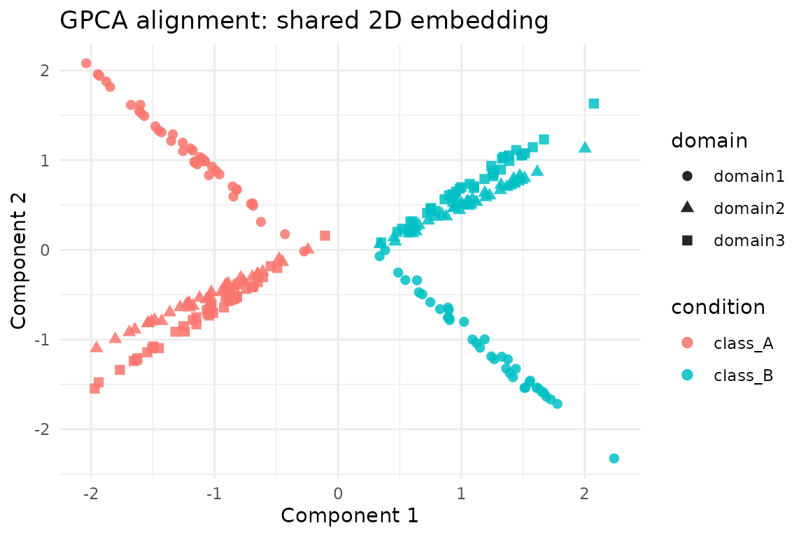

Controlling Graph Sparsification and Balancing

The optional control argument feeds through to gpca_align_control(), letting you adjust k-NN sparsification, label balancing and memory caps. Here we build a denser within-domain graph but down-weight the majority class via label balancing.

ctrl <- gpca_align_control(
  knn = 10,
  knn_mode = "mutual",
  balance = "within",
  balance_power = 0.5,
  normalize = "edges",
  verbose = FALSE
)

gpca_dense <- gpca_align(
  hd,
  y = condition,
  ncomp = 2,
  control = ctrl,
  preproc = base_preproc
)

summary(gpca_dense$sdev)
#>    Min. 1st Qu.  Median    Mean 3rd Qu.    Max. 
#>   5.633   5.703   5.773   5.773   5.843   5.912

When working with larger domains, consider leaving knn = NA (the default) to use fully dense metrics or lower the max_dense_elems parameter to enforce a safe memory ceiling. If gpca_align() detects that densifying the block matrix would exceed the limit, it aborts with a diagnostic message so you can tighten the sparsification or dimensionality reduction beforehand.

Next Steps

• gpca_align() returns a standard multivarious projector, so you can call predict() on new samples (via multivarious::multiblock_biprojector).
• The RMS alignment summary above shows how closely each domain pair agrees in the coupled space; values near zero indicate strong agreement.
• Use gpca_align_control() to add sparsification or label balancing when operating at larger scale.
• Pair gpca_align() with kema() or grasp() in the same pipeline to compare linear vs kernel alignment strategies.

This vignette is intentionally lightweight—swap in your own domains or expand chunks to benchmark larger settings.