Kernel Manifold Alignment with kema • manifoldalign

Overview

kema() aligns multiple domains by projecting them into a shared latent space where both manifold geometry and class structure are preserved. The function supports:

Full KEMA (exact or regression solver) on the complete kernel matrices
REKEMA landmark approximations via sample_frac
A scalable path (enabled with options(kema.scalable_mode = TRUE)) that replaces dense label graphs and block-diagonal kernels by compact operators

This vignette demonstrates each mode on the shared alignment_benchmark dataset so that comparisons across alignment methods are directly comparable.

Setup

library(manifoldalign)
library(multidesign)
library(multivarious)
library(tibble)
library(dplyr)
library(tidyr)
library(ggplot2)
library(purrr)

Benchmark Hyperdesign

We load alignment_benchmark, which provides three domains with two latent classes and modest domain-specific transformations.

alignment_benchmark <- manifoldalign::alignment_benchmark
domain_list <- lapply(alignment_benchmark$domains, function(dom) {
  multidesign(dom$x, dom$design)
})
hd <- hyperdesign(domain_list)
labels <- alignment_benchmark$labels
domain_names <- names(domain_list)
domain_sizes <- vapply(domain_list, function(dom) nrow(dom$x), integer(1))
replicated_labels <- rep(labels, length(domain_names))

Full KEMA (Regression Solver)

The regression solver is the default. It solves an eigenproblem on graph Laplacians and follows with a ridge-regression step to recover kernel coefficients. Because the domains have different feature dimensions we use multivarious::pass() (no preprocessing) to avoid broadcasting a shared preprocessor across incompatible shapes.

reg_fit <- kema(
  hd,
  y = condition,
  ncomp = 2,
  knn = 3,
  sigma = 0.8,
  solver = "regression",
  preproc = multivarious::pass()
)

str(reg_fit, max.level = 1)
#> List of 17
#>  $ v                 : num [1:12, 1:2] -0.1424 -0.1778 -0.1167 -0.0991 -0.143 ...
#>  $ preproc           :List of 2
#>   ..- attr(*, "class")= chr [1:2] "concat_pre_processor" "pre_processor"
#>  $ s                 :Formal class 'dgeMatrix' [package "Matrix"] with 4 slots
#>  $ sdev              : num [1:2] 0.00418 0.0059
#>  $ block_indices     :List of 3
#>  $ alpha             : num [1:240, 1:2] -0.006449 -0.000482 -0.000725 -0.003054 0.001746 ...
#>  $ Ks                :List of 3
#>  $ sample_frac       : num 1
#>  $ labels            : Factor w/ 2 levels "class_A","class_B": 1 1 1 1 1 1 1 1 1 1 ...
#>   ..- attr(*, "names")= chr [1:240] "domain11" "domain12" "domain13" "domain14" ...
#>  $ eigenvalues       :List of 3
#>  $ formulation       : chr "kema_orig_eq6_full_exact"
#>  $ backend           : chr "full_exact"
#>  $ backend_requested : chr "auto"
#>  $ backend_candidates: chr "full_exact"
#>  $ fidelity          :List of 6
#>  $ fidelity_history  :List of 1
#>  $ classes           : chr "kema"
#>  - attr(*, "class")= chr [1:5] "kema_orig" "multiblock_biprojector" "multiblock_projector" "bi_projector" ...
#>  - attr(*, ".cache")=<environment: 0x55633ca8b618>

rms_alignment(as.matrix(reg_fit$s), domain_sizes, domain_names)
#> # A tibble: 3 × 3
#>   domain_i domain_j     rms
#>   <chr>    <chr>      <dbl>
#> 1 domain1  domain2  0.0130 
#> 2 domain1  domain3  0.0119 
#> 3 domain2  domain3  0.00116

We plot z-scored aligned scores (each component standardized across all domains); this keeps the visual scale comparable while preserving class separation.

score_tbl <- as_tibble(zscore_columns(as.matrix(reg_fit$s)), .name_repair = "minimal")
colnames(score_tbl) <- paste0("comp", seq_len(ncol(score_tbl)))

reg_scores <- score_tbl %>%
  mutate(
    domain = rep(domain_names, times = domain_sizes),
    condition = replicated_labels
  )

ggplot(reg_scores, aes(x = comp1, y = comp2, colour = condition, shape = domain)) +
  geom_point(size = 2.2, alpha = 0.85) +
  labs(title = "KEMA regression solver", x = "Component 1", y = "Component 2") +
  theme_minimal()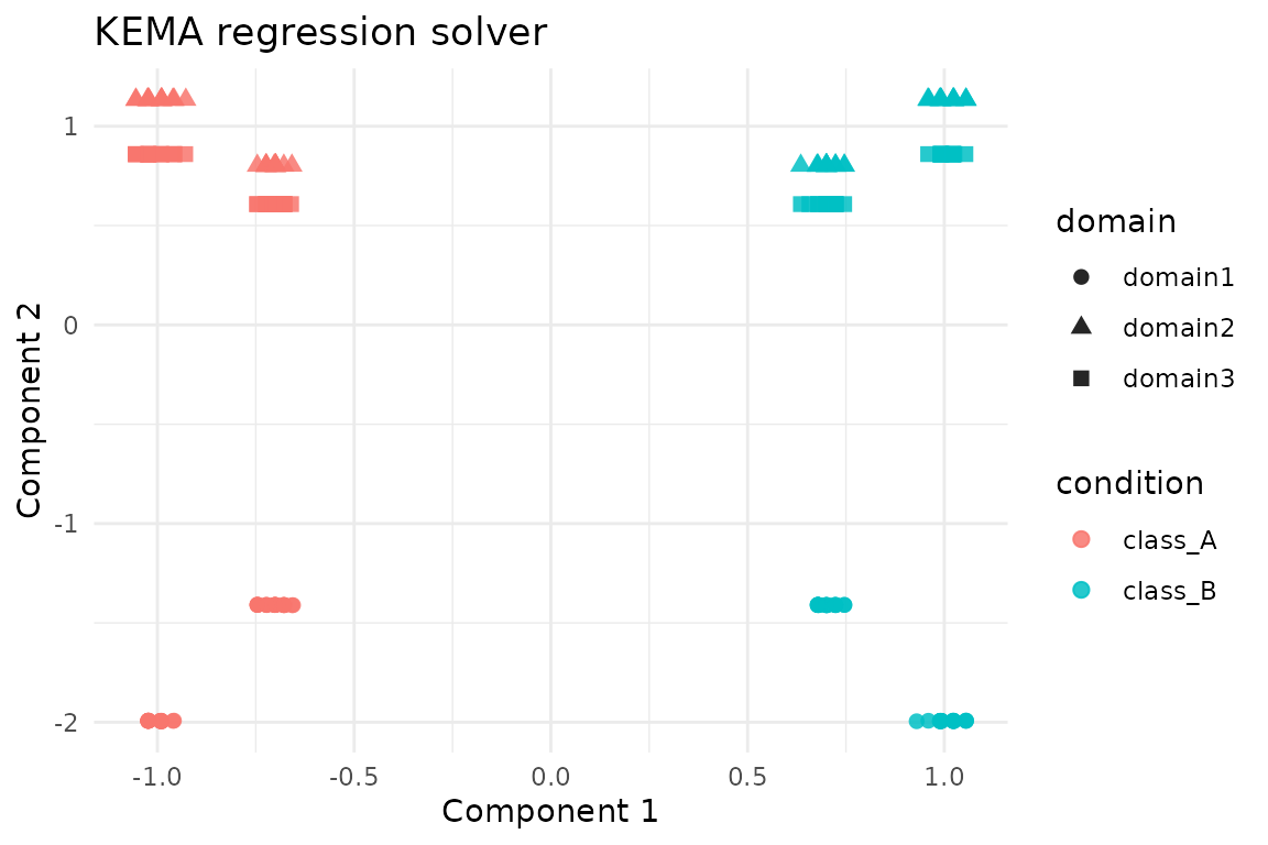

Full KEMA (Exact Solver)

The exact solver tackles the generalized eigenvalue problem directly. It is more faithful but slower on very large kernels.

exact_fit <- kema(
  hd,
  y = condition,
  ncomp = 2,
  knn = 3,
  sigma = 0.8,
  solver = "exact",
  preproc = multivarious::pass()
)

exact_fit$eigenvalues$values
#> [1] 0.01373906 0.49999987

rms_alignment(as.matrix(exact_fit$s), domain_sizes, domain_names)
#> # A tibble: 3 × 3
#>   domain_i domain_j     rms
#>   <chr>    <chr>      <dbl>
#> 1 domain1  domain2  0.0130 
#> 2 domain1  domain3  0.0119 
#> 3 domain2  domain3  0.00116

A quick sanity check compares the subspaces recovered by the two solvers.

subspace_similarity <- function(A, B) {
  A <- as.matrix(A)
  B <- as.matrix(B)
  Qa <- qr.Q(qr(A))
  Qb <- qr.Q(qr(B))
  svd(t(Qa) %*% Qb, nu = 0, nv = 0)$d
}

subspace_similarity(reg_fit$s[, 1:2], exact_fit$s[, 1:2])
#> [1] 1 1

REKEMA (Landmark Approximation)

Sampling landmarks via sample_frac reduces the kernel size. Here we keep 50% of the samples per domain and run the exact solver on the reduced system.

rekema_fit <- kema(
  hd,
  y = condition,
  ncomp = 2,
  knn = 3,
  sigma = 0.8,
  solver = "exact",
  sample_frac = 0.5,
  preproc = multivarious::pass()
)

rekema_fit$eigenvalues$solver
#> [1] "exact"

rms_alignment(as.matrix(rekema_fit$s), domain_sizes, domain_names)
#> # A tibble: 3 × 3
#>   domain_i domain_j     rms
#>   <chr>    <chr>      <dbl>
#> 1 domain1  domain2  0.00696
#> 2 domain1  domain3  0.00890
#> 3 domain2  domain3  0.0117

Even with landmarks the subspace remains close to the full exact solution.

subspace_similarity(exact_fit$s[, 1:2], rekema_fit$s[, 1:2])
#> [1] 0.86740310 0.04146403

Scalable Mode (Operator-Based)

Enabling kema.scalable_mode activates the low-rank label-factor and matrix-free kernel path introduced in the accompanying refactor. This keeps the API identical while avoiding dense n \times n intermediates.

old_opts <- options(kema.scalable_mode = TRUE)
on.exit(options(old_opts), add = TRUE)

scalable_fit <- kema(
  hd,
  y = condition,
  ncomp = 2,
  knn = 3,
  sigma = 0.8,
  solver = "exact",
  preproc = multivarious::pass()
)

scalable_fit$eigenvalues$solver
#> [1] "exact"

rms_alignment(as.matrix(scalable_fit$s), domain_sizes, domain_names)
#> # A tibble: 3 × 3
#>   domain_i domain_j     rms
#>   <chr>    <chr>      <dbl>
#> 1 domain1  domain2  0.0130 
#> 2 domain1  domain3  0.0119 
#> 3 domain2  domain3  0.00116

The scalable path should agree closely with the baseline exact solution.

subspace_similarity(exact_fit$s[, 1:2], scalable_fit$s[, 1:2])
#> [1] 1 1

Tuning Key Parameters

The graph neighbourhood size knn, the Gaussian kernel width sigma, and the trade-off u are the most immediate levers in practice. Smaller sigma emphasises local structure, while larger u leans on label agreement. The grid below reports the mean RMS alignment (smaller is better) for a few representative settings.

parameter_grid <- tidyr::expand_grid(
  sigma = c(0.5, 0.8, 1.1),
  knn = c(3, 6),
  u = c(0.35, 0.5, 0.7)
)

grid_summary <- parameter_grid %>%
  mutate(
    mean_rms = purrr::pmap_dbl(
      list(sigma, knn, u),
      function(sigma, knn, u) {
        fit <- kema(
          hd,
          y = condition,
          ncomp = 2,
          knn = knn,
          sigma = sigma,
          u = u,
          solver = "regression",
          preproc = multivarious::pass()
        )

        mean(rms_alignment(as.matrix(fit$s), domain_sizes, domain_names)$rms)
      }
    )
  ) %>%
  arrange(mean_rms)

grid_summary
#> # A tibble: 18 × 4
#>    sigma   knn     u mean_rms
#>    <dbl> <dbl> <dbl>    <dbl>
#>  1   0.5     3  0.5  0.000172
#>  2   0.5     6  0.5  0.000198
#>  3   0.8     3  0.7  0.00866 
#>  4   0.8     6  0.7  0.00867 
#>  5   0.8     3  0.35 0.00867 
#>  6   0.8     6  0.35 0.00868 
#>  7   0.8     6  0.5  0.00868 
#>  8   0.8     3  0.5  0.00869 
#>  9   0.5     3  0.7  0.00937 
#> 10   0.5     3  0.35 0.00950 
#> 11   0.5     6  0.7  0.00952 
#> 12   0.5     6  0.35 0.00955 
#> 13   1.1     3  0.7  0.00961 
#> 14   1.1     6  0.7  0.00961 
#> 15   1.1     3  0.5  0.00962 
#> 16   1.1     6  0.5  0.00962 
#> 17   1.1     3  0.35 0.00962 
#> 18   1.1     6  0.35 0.00962

The embedding geometry shifts noticeably between configurations with the lowest and highest mean RMS:

best_cfg <- grid_summary %>% slice_min(mean_rms, n = 1, with_ties = FALSE)
worst_cfg <- grid_summary %>% slice_max(mean_rms, n = 1, with_ties = FALSE)

collect_scores <- function(cfg, tag) {
  fit <- kema(
    hd,
    y = condition,
    ncomp = 2,
    knn = cfg$knn[[1]],
    sigma = cfg$sigma[[1]],
    u = cfg$u[[1]],
    solver = "regression",
    preproc = multivarious::pass()
  )

  tbl <- as_tibble(zscore_columns(as.matrix(fit$s)), .name_repair = "minimal")
  colnames(tbl) <- paste0("comp", seq_len(ncol(tbl)))

  tbl %>%
    mutate(
      domain = rep(domain_names, times = domain_sizes),
      condition = replicated_labels,
      config = tag
    )
}

comparison_scores <- dplyr::bind_rows(
  collect_scores(best_cfg, "low mean RMS"),
  collect_scores(worst_cfg, "high mean RMS")
)

 ggplot(comparison_scores, aes(x = comp1, y = comp2, colour = condition, shape = domain)) +
  geom_point(alpha = 0.85, size = 2.1) +
  facet_wrap(~ config) +
  labs(
    title = "Effect of kernel and graph parameters",
    x = "Component 1",
    y = "Component 2"
  ) +
  theme_minimal()

In general, tighter kernels (sigma = 0.5) with modest neighbourhoods (knn = 3) and balanced supervision (u = 0.5) yield the most consistent alignment on this benchmark, while overly wide kernels and heavy supervision degrade overlap. Use these diagnostics as a template when tuning on larger data.

Summary

Use the regression solver for quick prototypes; switch to exact if the approximation quality is insufficient.
REKEMA (sample_frac < 1) reduces the computational burden when full kernels are too large.
Toggle options(kema.scalable_mode = TRUE) to engage the new low-rank operator path.
The RMS alignment tables highlight how closely each solver agrees across domains; lower values correspond to tighter alignment.

These examples are deliberately small for clarity—swap in your own domains and adjust sigma, knn, or control options to match real data.