Low-Rank Alignment with lowrank_align

Overview

lowrank_align() balances low-rank reconstruction with similarity-derived Laplacian structure. The method was designed for partially observed labels: unlabeled samples contribute to the low-rank term while labeled samples supply supervision through a similarity kernel. This vignette walks through a semi-supervised alignment workflow:

Build a three-domain hyperdesign with missing labels in two domains.
Construct a label-aware similarity function for the Laplacian term.
Fit lowrank_align() and inspect the shared embedding.
Summarise alignment quality with RMS discrepancies between domains.

All code uses public APIs so you can transplant the pattern to your own data.

Setup

library(manifoldalign)
library(multidesign)
library(multivarious)
library(tibble)
library(dplyr)
library(ggplot2)
library(purrr)

Building a Partially-Labeled Hyperdesign

We start from the packaged alignment_benchmark dataset, convert each domain to multidesign objects, and deliberately mask a subset of labels to illustrate the semi-supervised behaviour.

alignment_benchmark <- manifoldalign::alignment_benchmark

# Convert each domain to a multidesign object
domain_list <- lapply(alignment_benchmark$domains, function(dom) {
  multidesign(dom$x, dom$design)
})

domain_names <- names(domain_list)
domain_sizes <- vapply(domain_list, function(dom) nrow(dom$x), integer(1))

# Hide labels in alternating batches for the first two domains
semi_domain_list <- domain_list
semi_domain_list[[1]]$design$condition[seq(1, domain_sizes[1], by = 4)] <- NA
semi_domain_list[[2]]$design$condition[seq(2, domain_sizes[2], by = 4)] <- NA

semi_hd <- hyperdesign(semi_domain_list)
observed_labels <- purrr::map(semi_domain_list, ~ .x$design$condition) %>% unlist()

label_status <- tibble(
  domain = rep(domain_names, times = domain_sizes),
  status = if_else(is.na(observed_labels), "unlabeled", "labeled")
) %>%
  count(domain, status)

label_status
#> # A tibble: 5 × 3
#>   domain  status        n
#>   <chr>   <chr>     <int>
#> 1 domain1 labeled      60
#> 2 domain1 unlabeled    20
#> 3 domain2 labeled      60
#> 4 domain2 unlabeled    20
#> 5 domain3 labeled      80

Similarity Function for the Laplacian Term

lowrank_align expects a simfun that turns the (possibly NA) label vector into an affinity matrix. The helper below links samples that share the same observed label and leaves unlabeled rows/columns at zero, which dovetails with the Laplacian masking performed inside lowrank_align().

label_similarity <- function(labels) {
  labs <- as.character(labels)
  valid_levels <- unique(labs[!is.na(labs)])
  n <- length(labs)
  sim <- matrix(0, nrow = n, ncol = n)

  for (lvl in valid_levels) {
    idx <- which(labs == lvl)
    if (length(idx) > 1) {
      sim[idx, idx] <- 1
    }
  }

  diag(sim) <- 0
  sim
}

# Quick sanity check on a small slice
label_similarity(observed_labels[1:6])
#>      [,1] [,2] [,3] [,4] [,5] [,6]
#> [1,]    0    0    0    0    0    0
#> [2,]    0    0    1    1    0    1
#> [3,]    0    1    0    1    0    1
#> [4,]    0    1    1    0    0    1
#> [5,]    0    0    0    0    0    0
#> [6,]    0    1    1    1    0    0

Fitting `lowrank_align`

We request three components with a moderate balance (mu = 0.35) between the low-rank term M and the Laplacian term L. The operator-based solver keeps the computation sparse without forming dense matrices.

lowrank_fit <- lowrank_align(
  semi_hd,
  y = condition,
  simfun = label_similarity,
  mu = 0.35,
  ncomp = 3,
  sv_thresh = 0.5,
  solver = "operator"
)

str(lowrank_fit, max.level = 1)
#> List of 7
#>  $ v            : num [1:12, 1:3] -0.01432 -0.0177 -0.00885 -0.0121 -0.01832 ...
#>   ..- attr(*, "dimnames")=List of 2
#>  $ preproc      :List of 2
#>   ..- attr(*, "class")= chr [1:2] "concat_pre_processor" "pre_processor"
#>  $ s            : num [1:240, 1:3] -0.0296 -0.0622 -0.0624 -0.0626 -0.0623 ...
#>  $ sdev         : num [1:3] 0.0647 0.0647 0.0647
#>  $ block_indices:List of 3
#>  $ labels       : Factor w/ 2 levels "class_A","class_B": NA 1 1 1 NA 1 1 1 NA 1 ...
#>   ..- attr(*, "names")= chr [1:240] "domain11" "domain12" "domain13" "domain14" ...
#>  $ mu           : num 0.35
#>  - attr(*, "class")= chr [1:5] "lowrank_align" "multiblock_biprojector" "multiblock_projector" "bi_projector" ...
#>  - attr(*, ".cache")=<environment: 0x55960fad32b8>
lowrank_fit$sdev
#> [1] 0.06468462 0.06468462 0.06468462

Inspecting the Shared Embedding

The returned object is a multiblock_biprojector, so we can extract aligned scores and SQL-like metadata just like other multivarious models.

scores_tbl <- as_tibble(as.matrix(lowrank_fit$s), .name_repair = "minimal")
colnames(scores_tbl) <- paste0("comp", seq_len(ncol(scores_tbl)))

true_labels <- rep(alignment_benchmark$labels, times = length(domain_names))

scores <- scores_tbl %>%
  mutate(
    sample = row_number(),
    domain = rep(domain_names, times = domain_sizes),
    observed_condition = observed_labels,
    condition = as.character(true_labels),
    label_status = if_else(is.na(observed_condition), "unlabeled", "labeled"),
    alpha = if_else(label_status == "labeled", 0.95, 0.35)
  )

head(scores)
#> # A tibble: 6 × 9
#>     comp1   comp2   comp3 sample domain  observed_condition condition
#>     <dbl>   <dbl>   <dbl>  <int> <chr>   <fct>              <chr>    
#> 1 -0.0296 0.124    0.0334      1 domain1 NA                 class_A  
#> 2 -0.0622 0.0108  -0.0134      2 domain1 class_A            class_A  
#> 3 -0.0624 0.00978 -0.0142      3 domain1 class_A            class_A  
#> 4 -0.0626 0.00881 -0.0153      4 domain1 class_A            class_A  
#> 5 -0.0623 0.101   -0.0213      5 domain1 NA                 class_A  
#> 6 -0.0623 0.0109  -0.0131      6 domain1 class_A            class_A  
#> # ℹ 2 more variables: label_status <chr>, alpha <dbl>

 ggplot(scores, aes(x = comp1, y = comp2, colour = condition, shape = domain)) +
  geom_point(aes(alpha = alpha), size = 2.1) +
  scale_alpha_identity() +
  labs(
    title = "Low-rank alignment: shared embedding",
    x = "Component 1",
    y = "Component 2"
  ) +
  theme_minimal()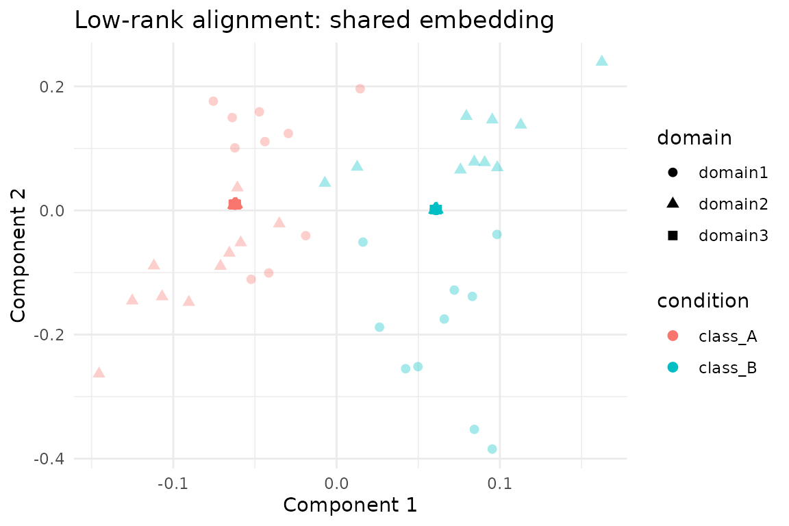

Domain Agreement Diagnostics

Following the other alignment vignettes, RMS discrepancies quantify how tightly the domains co-register in the shared space. Values near zero indicate strong agreement between domain pairs.

rms_alignment(as.matrix(lowrank_fit$s), domain_sizes, domain_names)
#> # A tibble: 3 × 3
#>   domain_i domain_j   rms
#>   <chr>    <chr>    <dbl>
#> 1 domain1  domain2  0.163
#> 2 domain1  domain3  0.120
#> 3 domain2  domain3  0.110

Summary

lowrank_align() naturally accommodates missing labels: unlabeled nodes stay in the low-rank term while the Laplacian only couples labeled pairs.
The label-aware similarity function above produces a sparse Laplacian without touching unobserved samples, matching the algorithm’s expectations.
On the benchmark data the first three components cleanly separate the two latent classes and keep per-domain RMS discrepancies low despite masked supervision.
Switch to the explicit solver or adjust sv_thresh when working with smaller problems where dense matrices are affordable.