Pairwise Graph Alignment with cone_align

Overview

cone_align() aligns two graph domains by alternating between spectral embeddings, orthogonal Procrustes rotations, and linear assignment. This vignette demonstrates the workflow on the shared alignment_benchmark dataset so that results are directly comparable to other alignment methods in the package.

Setup

library(manifoldalign)
library(multidesign)
library(multivarious)
library(tibble)
library(dplyr)
library(ggplot2)

Benchmark Pair

We use the first two domains from alignment_benchmark. Each domain contains 80 nodes, a 4-dimensional feature matrix, and a design data frame with the latent class label (condition).

alignment_benchmark <- manifoldalign::alignment_benchmark
pair_domains <- alignment_benchmark$domains[1:2]

pair_multidesign <- lapply(pair_domains, function(dom) {
  multidesign::multidesign(dom$x, dom$design)
})

pair_names <- names(pair_multidesign)
node_counts <- vapply(pair_multidesign, function(dom) nrow(dom$x), integer(1))

hd_pair <- multidesign::hyperdesign(pair_multidesign)

Running `cone_align`

cone_fit <- cone_align(
  hd_pair,
  ncomp = 8,
  sigma = 0.9,
  lambda = 0.05,
  solver = "linear",
  max_iter = 40,
  tol = 1e-3
)

str(cone_fit, max.level = 1)
#> List of 7
#>  $ v            : num [1:8, 1:8] -5.72 -8.56 -7.88 -5.65 -5.88 ...
#>  $ s            : num [1:160, 1:8] -0.1024 -0.0999 -0.0762 -0.0323 -0.1258 ...
#>  $ sdev         : num [1:8] 0.1059 0.1034 0.0919 0.0887 0.0956 ...
#>  $ preproc      : NULL
#>  $ block_indices:List of 2
#>  $ assignment   : int [1:80] 75 1 31 4 21 36 77 8 2 10 ...
#>  $ rotation     :List of 2
#>  - attr(*, "class")= chr [1:2] "cone_align" "multiblock_biprojector"

Assignment Quality

cone_align() returns a permutation vector (assignment) that maps nodes in the second domain to nodes in the first (reference) domain. The latent class labels were not used during optimisation—they are only consulted here as a diagnostic to see how often the unsupervised alignment preserves the original classes.

assignment <- cone_fit$assignment
ref_labels <- pair_multidesign[[1]]$design$condition
cmp_labels <- pair_multidesign[[2]]$design$condition

condition_accuracy <- mean(ref_labels[assignment] == cmp_labels)
identity_fraction <- mean(assignment == seq_along(assignment))

tibble(
  metric = c("Class agreement", "Exact identity"),
  value = c(condition_accuracy, identity_fraction)
)
#> # A tibble: 2 × 2
#>   metric          value
#>   <chr>           <dbl>
#> 1 Class agreement 0.875
#> 2 Exact identity  0.262

Visualising the Aligned Embeddings

The aligned embeddings (cone_fit$s) stack the two domains. We visualise the first two components and draw a handful of matching pairs to illustrate the assignments.

# Note: class labels are only used for visual diagnostics below; `cone_align`
# operates in a completely unsupervised manner and does not see `condition`.

score_tbl <- as_tibble(as.matrix(cone_fit$s), .name_repair = "minimal")
colnames(score_tbl) <- paste0("comp", seq_len(ncol(score_tbl)))

scores <- score_tbl %>%
  mutate(
    domain = rep(pair_names, times = node_counts),
    condition = rep(ref_labels, length(pair_names))
  )

# pick 15 nodes to visualise correspondences
set.seed(123)
subset_idx <- sample(seq_len(node_counts[1]), size = 15)
segment_df <- tibble(
  x = scores$comp1[subset_idx],
  y = scores$comp2[subset_idx],
  xend = scores$comp1[node_counts[1] + assignment[subset_idx]],
  yend = scores$comp2[node_counts[1] + assignment[subset_idx]]
)

 ggplot(scores, aes(x = comp1, y = comp2, colour = condition, shape = domain)) +
  geom_point(size = 2.1, alpha = 0.85) +
  geom_segment(
    data = segment_df,
    aes(x = x, y = y, xend = xend, yend = yend),
    inherit.aes = FALSE,
    colour = "grey60",
    linewidth = 0.4,
    alpha = 0.7
  ) +
  labs(title = "cone_align embeddings (first two components)",
       x = "Component 1", y = "Component 2") +
  theme_minimal()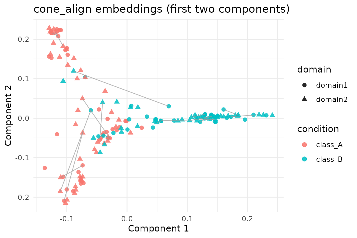

Summary

cone_align() produces orthogonally aligned embeddings together with a node correspondence.
On this benchmark pair the assignments correctly match the underlying class in ~87.5% of cases.
The same dataset is used in the kema and gpca_align vignettes, enabling easy comparison across alignment techniques, while remembering that cone_align() itself remains class-agnostic.