Validate and choose a reference model

library(referent)
reference <- ref_simulate(400, kind = "gaussian", scale = "age", seed = 1)
validation <- ref_simulate(300, kind = "gaussian", scale = "age", seed = 8)

The first model that converges is not necessarily a trustworthy reference. You need to decide how much distributional flexibility the data support and then test the chosen model on people who did not fit it. This page keeps those two jobs separate: cross-fitting chooses a candidate within the reference cohort; a held-out validation cohort checks the final fit.

Which distributional model earns its complexity?

Order candidates from the simplest plausible model to more flexible ones. Every ref_select() criterion is computed from out-of-fold predictions, so a candidate cannot win by explaining the same rows that fitted it.

ladder <- list(
  gaussian_constant = ref_spec(
    ref_gaussian(), location = ~ s(age, k = 8) + sex
  ),
  gaussian_varying_scale = ref_spec(
    ref_gaussian(), location = ~ s(age, k = 8) + sex,
    scale = ~ s(age, k = 5)
  ),
  shash_varying_scale = ref_spec(
    ref_shash(), location = ~ s(age, k = 8) + sex,
    scale = ~ s(age, k = 5)
  )
)
selection <- ref_select(ladder, reference, outcomes = "y", folds = 4)
selection$comparison[, c(
  "model", "mean_log_score", "crps", "mean_z", "var_z",
  "cover_95", "calibrated", "selected"
)]
#> # A tibble: 3 × 8
#>   model          mean_log_score  crps  mean_z var_z cover_95 calibrated selected
#>   <chr>                   <dbl> <dbl>   <dbl> <dbl>    <dbl> <lgl>      <lgl>
#> 1 gaussian_cons…          -1.88 0.891 0.0103  0.998    0.942 FALSE      FALSE
#> 2 gaussian_vary…          -1.85 0.889 0.00529 1.03     0.935 TRUE       TRUE
#> 3 shash_varying…          -1.86 0.892 0.00347 1.04     0.942 TRUE       FALSE

Read the table as a sequence of gates. Failed or unstable fits leave first. Calibration is checked before log score and CRPS. The paired one-standard-error rule then keeps candidates whose predictive performance is not distinguishable from the best, and the simplest survivor wins. A selected model is the most defensible member of this ladder, not proof that the ladder contained truth. Fold-specific support checks can mask a few boundary rows when one fold’s training range is narrower than the full reference range; the comparison reports the finite out-of-fold scoring set rather than filling those values.

How do you validate the selected model honestly?

Fit the selected specification to all reference rows, then assess a separate cohort. Declare the uncertainty regime explicitly so the reported diagnostics can be reproduced from predict().

fit <- ref_fit(selection$selected, reference, outcomes = "y")
assessment <- ref_assess(fit, validation, uncertainty = "total")
assessment$overall[, c(
  "mean_log_score", "standardized_log_score", "crps", "smse", "ev", "rmse"
)]
#> # A tibble: 1 × 6
#>   mean_log_score standardized_log_score  crps  smse    ev  rmse
#>            <dbl>                  <dbl> <dbl> <dbl> <dbl> <dbl>
#> 1          -1.82                  0.334 0.850 0.562 0.437  1.56
assessment$marginal[, c(
  "n", "mean_z", "var_z", "cover_50", "cover_80", "cover_95", "cover_99"
)]
#> # A tibble: 1 × 7
#>       n mean_z var_z cover_50 cover_80 cover_95 cover_99
#>   <int>  <dbl> <dbl>    <dbl>    <dbl>    <dbl>    <dbl>
#> 1   294 0.0265 0.909    0.517    0.833    0.966    0.993

mean_z and var_z diagnose location and spread on the normal-score scale. Coverage checks several central intervals. Log score and CRPS assess the full distribution rather than only its median. Compare models on the same held-out rows and uncertainty regime.

Where is the distribution wrong?

autoplot(assessment, type = "calibration")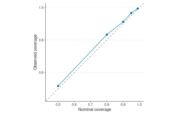

Points near the diagonal indicate marginal coverage. Departures identify which interval widths miss their nominal rates, but they do not reveal whether the error changes with age, sex, or site.

autoplot(assessment, type = "worm")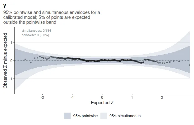

A tilted worm suggests a scale error; curvature suggests skew or tail misfit. Treat that shape as a diagnosis to test, not automatic permission to add a more flexible family. The QQ plot shows the same ordered scores against the standard normal without the detrending, which makes gross tail departures easier to see and small ones harder.

autoplot(assessment, type = "qq")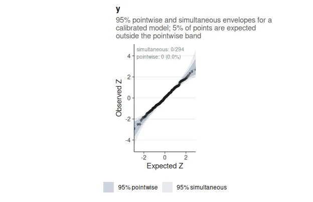

The tail table quantifies what the plot shows: observed versus expected exceedance rates at several tail levels, with standard errors.

assessment$tail
#> # A tibble: 4 × 6
#>   .outcome tail_level expected observed     n      se
#>   <chr>         <dbl>    <dbl>    <dbl> <int>   <dbl>
#> 1 y             0.005    0.005  0.00340   294 0.00411
#> 2 y             0.01     0.01   0.00680   294 0.00580
#> 3 y             0.025    0.025  0.0204    294 0.00911
#> 4 y             0.05     0.05   0.0340    294 0.0127

Does calibration drift across covariates or groups?

The conditional table checks every covariate used by the fit. Numeric covariates receive light diagnostic smooths; factors receive one row per level. The p-values test no drift, while the drift columns describe its size.

assessment$conditional[, c(
  ".outcome", "covariate", "level", "n",
  "location_drift", "location_p", "scale_drift", "scale_p"
)]
#> # A tibble: 3 × 8
#>   .outcome covariate level     n location_drift location_p scale_drift scale_p
#>   <chr>    <chr>     <chr> <int>          <dbl>      <dbl>       <dbl>   <dbl>
#> 1 y        age       <NA>    294        0.166        0.129      0.336    0.228
#> 2 y        sex       F       145        0.0525       0.510     -0.0798   0.472
#> 3 y        sex       M       149        0.00117      0.988     -0.108    0.277

If you ask for by = site, the marginal table is also split by site. Do this only when each group has enough held-out rows to estimate coverage and tails.

by_site <- ref_assess(fit, validation, by = site, uncertainty = "total")
by_site$marginal[, c(".group", "n", "mean_z", "var_z", "cover_95")]
#> # A tibble: 4 × 5
#>   .group     n   mean_z var_z cover_95
#>   <chr>  <int>    <dbl> <dbl>    <dbl>
#> 1 A         81  0.123   0.700    0.988
#> 2 B         57 -0.0128  1.07     0.930
#> 3 C         77 -0.0197  1.08     0.961
#> 4 D         79  0.00119 0.860    0.975

What should happen after a failed check?

Do not tune and validate on the same rows. Revise the candidate ladder or covariates using reference-only cross-fitting, then return once to an untouched validation cohort. If failure is concentrated at a new scanner, use a transport analysis instead of bending the shared trajectory to that scanner. If scores are missing, diagnose support before model complexity.

Continue with Brain charts across sites (vignette("brain-charts-across-sites", package = "referent")), or use Troubleshooting reference models when a fit or score does not behave as expected.