Getting started with referent

library(referent)

You have a reference cohort, an outcome such as a regional brain volume, and covariates that explain ordinary population variation. You want to place new observations in the distribution expected for people with those covariates. This page takes one default path from those inputs to an interpretable score.

A reference model estimates the full conditional distribution, not just a mean curve. A centile is the distribution’s CDF at the observed value; z is qnorm(centile); and tail_prob is the smaller tail. None of them is a clinical label.

FAQ: choosing covariates and a reference population

These decisions are made before the first ref_fit() call and no function in the package makes them for you. The answers below are the defaults a careful analyst would reach for; each links to the place where the package gives you the evidence to revise them.

Which covariates? Age and sex are the usual conditioning set for a brain chart: they explain ordinary population variation you do not want to call a deviation. Put age in a smooth, s(age, k = 8), and sex as a factor. Anything you add becomes part of the question the score answers: conditioning on education, for example, turns “is this volume unusual for a 60-year-old woman?” into “… for a 60-year-old woman with this much education”, which may or may not be what you want to know.

Site as a random effect, not a covariate. Scanners shift measurements, but a new participant may come from a scanner that contributed no reference rows. s(site, bs = "re") estimates a shrunk level per site and returns the population curve for an unseen level (reported as support == "new_group"), while a fixed site factor has no prediction at all for a level it never saw. Brain charts across sites covers the transport choices that follow.

Head size: covariate or offset? A covariate log(icv) lets the data decide how volume scales with intracranial volume; the score then asks whether the volume is unusual for that head size. An offset, offset(log(icv)) under transform = "log", fixes the scaling at proportional and scores the volume as a fraction of head size. The two differ when the scaling is not proportional (it usually is not, across regions), and they answer different questions: prefer the covariate unless you have a reason to assert proportionality.

proportions <- ref_simulate(400, seed = 11)
proportions$icv <- exp(rnorm(nrow(proportions), 14, 0.1))
proportions$volume <- exp(0.8 * log(proportions$icv) + 0.02 * proportions$age +
                            rnorm(nrow(proportions), 0, 0.05))
as_covariate <- ref_spec(ref_gaussian(), ~ s(age, k = 6) + sex + log(icv),
                         transform = "log")
as_offset <- ref_spec(ref_gaussian(), ~ s(age, k = 6) + sex + offset(log(icv)),
                      transform = "log")
rbind(
  covariate = tidy(ref_fit(as_covariate, proportions, "volume"))[, c("status", "edf")],
  offset = tidy(ref_fit(as_offset, proportions, "volume"))[, c("status", "edf")]
)

# A tibble: 2 × 2
  status   edf
* <chr>  <dbl>
1 ok      4.00
2 ok      3.00

Both fit; the offset model spends one parameter fewer because it never estimates the slope on log(icv), and it is misspecified here because the true exponent is 0.8, not 1.

Who belongs in the reference? Everyone whose distribution you want to call “expected”. A reference of healthy controls gives scores relative to health; a population-based reference includes the prevalence of disease in that population. The package never decides this because no covariate column can encode the decision: write the inclusion rule down, apply it before ref_fit(), and record it in ref_freeze(criteria = ) so it travels with the reference.

How many local controls does ref_adapt() need? Adaptation estimates a location offset and, optionally, a log-scale offset, each shrunk toward zero by a ridge worth location_prior_n and scale_prior_n pseudo-observations. The location offset is a shrunk mean residual: with 30 controls its standard error is about 1 / sqrt(30), or 0.18 in z units, and it is usable with far fewer. The scale offset needs several times more, because the variance of a variance estimate is larger. The site-transport comparison sets out that arithmetic for 30 controls, and its conclusion is the general one: adapt location first, adapt scale only when local n justifies it, and calibrate by site only with still more.

What does |z| > 2 mean? Under a calibrated model, 4.55% of rows from the reference population exceed it by chance, so the count you observe is only informative against that expectation. ref_flag() reports it as the expected_exceedances attribute alongside the observed count and an FDR-adjusted tail probability per row. A flagged row is an exceedance with a known chance rate, not a diagnosis.

Gaussian or SHASH? Start Gaussian. Switch to ref_shash() when held-out scores are skewed or heavy-tailed (skew_z and excess_kurtosis_z in ref_assess()$marginal), and let ref_select() arbitrate: its calibration gate removes candidates whose out-of-fold coverage and tail rates are wrong, and its one-standard-error rule keeps the simplest model that predicts as well as the best. A SHASH fit can also let skew and tail weight vary with a covariate. Use that flexibility sparingly; it is estimated from the tails of the data, where there is least information.

skewed <- ref_simulate(400, kind = "shash", skew = 0.6, tail = 1, seed = 12)
shape_spec <- ref_spec(
  family = ref_shash(),
  location = ~ s(age, k = 6) + sex,
  scale = ~ s(age, k = 5),
  skew = ~ s(age, k = 4),
  tail = ~ 1
)
shape_fit <- ref_fit(shape_spec, skewed, outcomes = "y")
shape_fit

<ref_fit> shash via mgcv

1 outcome, n = 400

covariates: age and sex

status: ok=1

Read further in Validate and choose a reference model (vignette("validate-reference", package = "referent")).

What data do you need?

The reference rows define the population. Target rows are the observations you will score. Here both are deterministic simulations with an age trend, sex effect, and age-dependent spread.

reference <- ref_simulate(400, kind = "gaussian", scale = "age", seed = 1)
target <- ref_simulate(150, kind = "gaussian", scale = "age", seed = 5)
head(reference[, c("age", "sex", "site", "y")])

       age sex site         y
1 35.93052   F    C  8.267211
2 42.32743   F    A 11.200172
3 54.37120   F    D 11.116406
4 74.49247   M    D 12.784176
5 32.10092   F    A  8.083688
6 73.90338   M    C  9.606036

In your data, use stable participant identifiers and fit only on rows that belong to the declared reference population. referent never decides who belongs in that population for you.

How do you fit and score the first model?

ref_spec() declares one formula for each distributional parameter. ref_fit() fits that specification, and predict() places held-out rows in the fitted distribution.

spec <- ref_spec(
  family = ref_gaussian(),
  location = ~ s(age, k = 8) + sex,
  scale = ~ s(age, k = 5)
)
fit <- ref_fit(spec, data = reference, outcomes = "y")
target <- target[ref_support(fit, target)$support == "in", ]
scores <- predict(fit, newdata = target, type = "scores")
scores[1:5, c(".id", "observed", "median", "centile", "z", "tail_prob", "support")]

<ref_scores> 5 rows

# A tibble: 5 × 7
    .id observed median  centile      z tail_prob support
  <int>    <dbl>  <dbl>    <dbl>  <dbl>     <dbl> <chr>
1     1     8.09   8.33 0.429    -0.180  0.857    in
2     2     7.85  10.4  0.0655   -1.51   0.131    in
3     3    10.5   11.2  0.366    -0.342  0.733    in
4     4     8.14   9.23 0.203    -0.831  0.406    in
5     5     3.34   7.79 0.000488 -3.30   0.000976 in

Read one row as a chain: observed is the measurement, median is the reference model’s central prediction, centile is its conditional rank, and z expresses that rank on a standard-normal scale. support says whether the covariates justify interpolation.

What does the fitted chart show?

autoplot(fit, type = "centiles", by = sex, newdata = target)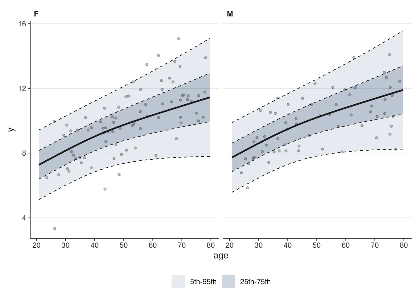

Notice that the bands widen with age because the scale formula varies with age. The points are held out: the figure shows how new observations sit in the reference distribution, not how closely the model redraws its training data. It is a calibration aid, not evidence that the reference cohort is clinically appropriate.

When should you trust a score?

Support is part of the result, not an optional diagnostic. By default, referent masks probability scores outside the reference covariate range, for missing predictors, and for unseen factor levels.

edge_cases <- target[1:3, ]
edge_cases$age <- c(median(reference$age), max(reference$age) + 20, NA_real_)
ref_support(fit, edge_cases)[, c("support", "d2")]

# A tibble: 3 × 2
  support       d2
  <chr>      <dbl>
1 in       0.00476
2 out      9.03
3 unknown NA

predict(fit, edge_cases)[, c(".id", "z", "support", "status")]

<ref_scores> 3 rows

# A tibble: 3 × 4
    .id     z support status
  <int> <dbl> <chr>   <chr>
1     1 -1.07 in      ok
2     2 NA    out     ok
3     3 NA    unknown missing_predictor

Do not remove the mask just to obtain a number. First decide whether the row is a data error, needs a better reference cohort, or belongs to a documented transport analysis. The troubleshooting article (vignette("troubleshooting", package = "referent")) shows those recovery paths.

How do you use the predictive distribution directly?

predict(type = "distribution") returns a distributional vector per outcome. The same object supplies centiles, intervals, simulation, and scores, so those summaries cannot silently drift apart.

dists <- predict(fit, target[1:3, ], type = "distribution",
                 uncertainty = "conditional")$y
hilo(dists, 90)

<hilo[3]>
[1] [6.197536, 10.47722]90 [7.641887, 13.18233]90 [7.779167, 14.60038]90

as_scores(dists, target$y[1:3])[, c("centile", "z", "tail_prob")]

# A tibble: 3 × 3
  centile      z tail_prob
    <dbl>  <dbl>     <dbl>
1  0.425  -0.189     0.850
2  0.0642 -1.52      0.128
3  0.365  -0.346     0.729

generate() draws synthetic observations from the same distributions, which is how you simulate a reference-like cohort with given covariates, for a power calculation or to check a downstream pipeline on data with no real participants in it.

set.seed(1)
synthetic <- generate(dists, times = 4)
synthetic

[[1]]
[1]  7.522404  8.576285  7.250282 10.412729

[[2]]
[1] 10.967055  9.030295 11.233022 11.655574

[[3]]
[1] 12.38366 10.55655 14.32445 11.99811

Does the model deserve interpretation?

Assess on rows that were not used for fitting. Here uncertainty = "total" matches the default score call above and includes uncertainty in the fitted curves.

assessment <- ref_assess(fit, target, uncertainty = "total")
assessment$marginal[, c("n", "mean_z", "var_z", "cover_50", "cover_95")]

# A tibble: 1 × 5
      n   mean_z var_z cover_50 cover_95
  <int>    <dbl> <dbl>    <dbl>    <dbl>
1   139 -0.00745 0.926    0.511    0.957

assessment$overall[, c("mean_log_score", "crps", "rmse")]

# A tibble: 1 × 3
  mean_log_score  crps  rmse
           <dbl> <dbl> <dbl>
1          -1.82 0.844  1.50

A calibrated model has mean_z near 0, var_z near 1, and observed coverage near its nominal level. Those are sampling targets, not exact pass/fail values for one small data set. Use the validation workflow next when you need model selection, conditional diagnostics, and tail checks.

What should you report about large deviations?

flags <- ref_flag(scores, threshold = 2)
c(
  observed = attr(flags, "observed_exceedances"),
  expected = attr(flags, "expected_exceedances")
)

observed expected
6.000000 6.324537

A large |z| can mean a genuinely unusual observation, unsupported covariates, or a miscalibrated model. Report the reference definition, held-out calibration, support status, and expected exceedance count before interpreting any flagged row.

Continue with Validate and choose a reference model. For site transport, go to Brain charts across sites.