Longitudinal change
A cross-sectional chart is a trajectory of distributions, not a distribution of trajectories. It says what the population looks like at each age; it says nothing about how one person moves from one visit to the next. People track centiles, and whether a follow-up value is surprising depends on how strongly their earlier values predict it.
referent treats this as a dynamic extension of the reference model.
The marginal fit maps each visit to a normal score
Z = qnorm(F(y | x)); a Gaussian process on those scores describes
within-person dependence across time; everything longitudinal is then a
conditional distribution under that process.
library(referent)Longitudinal reference data
Section titled “Longitudinal reference data”Subjects have two to four visits at irregular intervals. The normal
score of y is generated as a stable subject component plus a
Matern-3/2 process in time plus measurement noise, with variance
fractions 0.5, 0.35, and 0.15.
long <- ref_simulate(1200, kind = "longitudinal", seed = 1)truth <- attr(long, "truth")c(stable = truth$tau_b^2, dynamic = truth$tau_g^2, measurement = truth$sigma_e^2, ell = truth$ell)#> stable dynamic measurement ell#> 0.50 0.35 0.15 5.00head(long[, c("participant_id", "visit", "age", "sex", "y")])#> participant_id visit age sex y#> 1 1 1 69.77699 F 12.532202#> 2 1 2 71.34786 F 12.644226#> 3 2 1 71.68352 F 10.732819#> 4 2 2 74.49880 F 10.359598#> 5 2 3 75.59911 F 9.215615#> 6 2 4 76.77882 F 9.576045The marginal reference, then the process
Section titled “The marginal reference, then the process”The marginal model is the usual cross-sectional fit. ref_dynamics()
then estimates the process on total-uncertainty normal scores. By default it uses
out-of-fold scores from a subject-level cross-fit, so that in-sample
shrinkage does not masquerade as within-person dependence. The chosen
uncertainty mode and draw count are stored on dyn and reused by every
transition and forecast.
spec <- ref_spec(ref_gaussian(), location = ~ s(age, k = 6) + sex, scale = ~1)fit <- ref_fit(spec, data = long, outcomes = "y", id = participant_id)dyn <- ref_dynamics(fit, data = long, id = participant_id, time = age)dyn#> <ref_dynamics> 1 outcome; requested kernel: matern32; Z: out_of_fold, total#> uncertainty#> kernel uncertainty: plug-in (not propagated)#> subjects: 400; time range [20.07, 77.23]; lag range [0.502, 8.22]#> # A tibble: 1 × 12#> .outcome process identified at_boundary stable dynamic measurement ell#> <chr> <chr> <lgl> <lgl> <dbl> <dbl> <dbl> <dbl>#> 1 y matern32 TRUE FALSE 0.705 0.180 0.115 2.55#> # ℹ 4 more variables: ell_identified <lgl>, median_lag <dbl>,#> # r_median_lag <dbl>, r_median_lag_se <dbl>The print shows the estimated variance fractions of the stable, dynamic,
and measurement components, the correlation at the median lag with a
standard error, and the Matern length-scale. The components table
holds the same numbers.
dyn$components#> # A tibble: 1 × 12#> .outcome process identified at_boundary stable dynamic measurement ell#> <chr> <chr> <lgl> <lgl> <dbl> <dbl> <dbl> <dbl>#> 1 y matern32 TRUE FALSE 0.705 0.180 0.115 2.55#> # ℹ 4 more variables: ell_identified <lgl>, median_lag <dbl>,#> # r_median_lag <dbl>, r_median_lag_se <dbl>The kernel plot is the implied correlation between two normal scores of the same person as a function of the time between them. The jump at lag zero is the measurement nugget; the plateau is the stable rank.
autoplot(dyn, type = "kernel")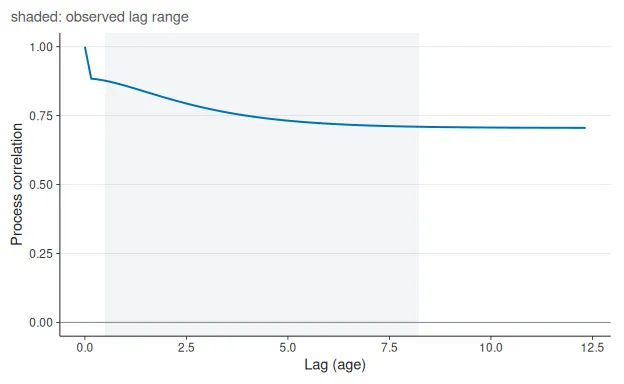
Identifiability and the stable model
Section titled “Identifiability and the stable model”Three components cannot be separated from two-visit data at one fixed
interval. With a single lag, any dependence structure collapses to one
number, the correlation at that lag, and the Matern length-scale is not
identified. ref_dynamics() detects this and reduces to the stable
model (ref_process("stable")): a subject intercept plus nugget, one
parameter. Everything downstream still works; it just cannot
extrapolate to other intervals, and forecasts at other lags are flagged
extrapolated_lag.
two_visit <- long[long$visit <= 2, ]two_visit <- two_visit[ave(two_visit$visit, two_visit$participant_id, FUN = length) == 2, ]two_visit$age <- ave(two_visit$age, two_visit$participant_id, FUN = function(a) a[1] + 2 * (seq_along(a) - 1))dyn_fixed <- ref_dynamics(fit, data = two_visit, id = participant_id, time = age, crossfit = 0)dyn_fixed$components[, c("process", "identified", "ell_identified", "median_lag", "r_median_lag")]#> # A tibble: 1 × 5#> process identified ell_identified median_lag r_median_lag#> <chr> <lgl> <lgl> <dbl> <dbl>#> 1 stable TRUE FALSE 2 0.823Separating measurement noise from rank dynamics needs either short
repeat intervals or three or more visits per subject;
dyn$identifiability$measurement records whether that was possible.
When too few subjects have repeats, the process is reported as not
identified and every history-conditioned quantity downstream is NA.
one_visit <- long[!duplicated(long$participant_id), ]dyn_unidentified <- ref_dynamics( fit, data = one_visit, id = participant_id, time = age, crossfit = 0)dyn_unidentified$components[, c("identified", "process", "r_median_lag")]#> # A tibble: 1 × 3#> identified process r_median_lag#> <lgl> <chr> <dbl>#> 1 FALSE matern32 NAThe fix is a stronger repeated-measures design, not an optimizer switch. Add participants with repeated visits and informative lag variation; do not report history-conditioned change from a cross-sectional sample.
Six longitudinal quantities
Section titled “Six longitudinal quantities”The design separates six questions that are often conflated.
| Quantity | Question | Where |
|---|---|---|
| Chart velocity | How does a reference centile itself move with age? | ref_derivative() |
| Observed velocity | At what raw rate did this person change? | ref_transition()$observed_velocity |
| Expected velocity | What rate was expected given this person’s history? | ref_transition()$expected_velocity |
| Velocity centile | Where does the observed rate fall in the conditional distribution? | ref_transition()$velocity_centile |
| Innovation Z | How surprising is the follow-up after conditioning on history? | ref_transition()$innovation_z |
| Change Z | How unusual is the change in the unconditional distribution of changes? | ref_transition()$change_z |
Chart velocity is a property of the population curve, not of any person:
grid <- data.frame(age = c(30, 50, 70), sex = factor("F", levels = c("F", "M")))ref_derivative(fit, grid, with_respect_to = age, centiles = c(0.1, 0.5, 0.9))#> # A tibble: 9 × 5#> .outcome time centile chart_velocity chart_velocity_se#> * <chr> <dbl> <dbl> <dbl> <dbl>#> 1 y 30 0.1 0.112 0.0101#> 2 y 50 0.1 0.0703 0.00888#> 3 y 70 0.1 0.0359 0.0163#> 4 y 30 0.5 0.112 0.0101#> 5 y 50 0.5 0.0703 0.00888#> 6 y 70 0.5 0.0359 0.0163#> 7 y 30 0.9 0.112 0.0101#> 8 y 50 0.9 0.0703 0.00888#> 9 y 70 0.9 0.0359 0.0163The others come from ref_transition(), one row per consecutive pair
of visits. Innovation Z is the history-conditioned score
(Z_2 - m) / s, where m and s are the conditional mean and SD of
the new score given all earlier ones; with one prior visit it reduces
to the Z-gain (Z_2 - r Z_1) / sqrt(1 - r^2). Change Z is the
difference Z_2 - Z_1 standardised by its own SD sqrt(2(1 - r)).
Both are N(0, 1) under the reference process; the naive difference
Z_2 - Z_1 is not.
held <- ref_simulate(2400, kind = "longitudinal", seed = 7)tr <- ref_transition(dyn, data = held, id = participant_id, time = age)tr[1:4, c(".id", ".dt", "observed_velocity", "expected_velocity", "velocity_centile", "innovation_z", "change_z", "support")]#> <ref_transition> 4 transitions#> # A tibble: 4 × 8#> .id .dt observed_velocity expected_velocity velocity_centile innovation_z#> <int> <dbl> <dbl> <dbl> <dbl> <dbl>#> 1 1 1.23 0.672 0.302 0.739 0.639#> 2 1 0.646 -2.47 -0.124 0.00755 -2.43#> 3 2 2.34 -0.269 0.108 0.136 -1.10#> 4 2 2.27 0.216 0.270 0.438 -0.157#> # ℹ 2 more variables: change_z <dbl>, support <chr>On held-out subjects from the same generator both scores are calibrated,
and the rate of |z| > 1.96 is near 5%. The naive difference is not.
naive <- with(tr, qnorm(end_centile) - qnorm(start_centile))rbind( innovation = c(var = var(tr$innovation_z, na.rm = TRUE), fpr = mean(abs(tr$innovation_z) > 1.96, na.rm = TRUE)), change = c(var = var(tr$change_z, na.rm = TRUE), fpr = mean(abs(tr$change_z) > 1.96, na.rm = TRUE)), naive = c(var = var(naive, na.rm = TRUE), fpr = mean(abs(naive) > 1.96, na.rm = TRUE)))#> var fpr#> innovation 1.0469679 0.059720457#> change 1.0411358 0.055908513#> naive 0.3587321 0.001270648autoplot(dyn, type = "calibration", data = held, id = participant_id, time = age)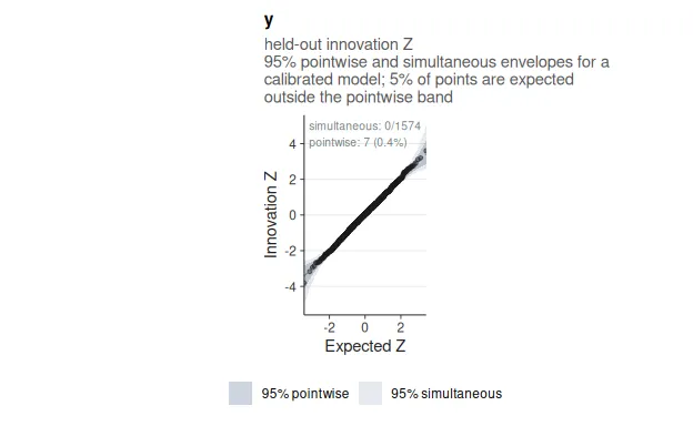
autoplot(tr, type = "innovation")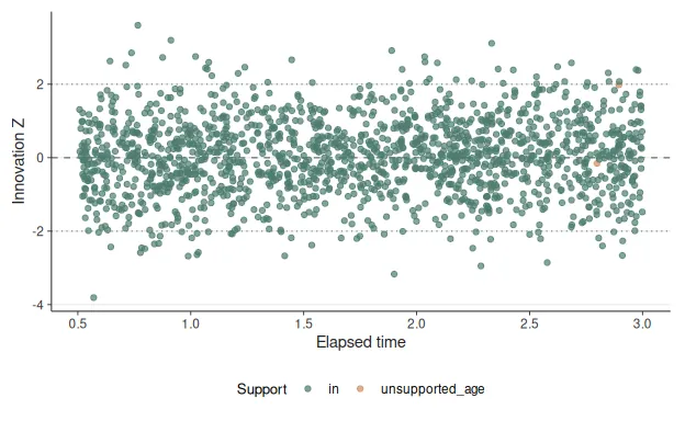
The thrive plot is the population-level view of the same process. Each
line starts on a reference centile and follows the thrive conditional
quantile (by default 0.025) of the forecast horizon time units later: a
follow-up below that line is unexpectedly low given where the person
started, which is what innovation Z measures. Because the process regresses
toward the mean, the lines run toward the median, and a person who merely
crosses a centile line has not necessarily changed more than expected.
autoplot(dyn, type = "thrive", horizon = 2)#> `geom_line()`: Each group consists of only one observation.#> ℹ Do you need to adjust the group aesthetic?#> `geom_line()`: Each group consists of only one observation.#> ℹ Do you need to adjust the group aesthetic?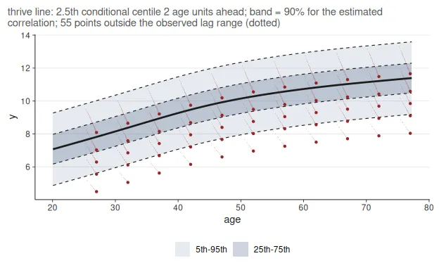
Forecasts
Section titled “Forecasts”ref_forecast() conditions the marginal distribution at future times
on a subject’s history and returns one dist_conditioned() predictive
distribution per time. The fan starts at the last observed visit; its
width at short horizons reflects the measurement nugget and grows toward
the marginal spread as the dynamic component decorrelates. Times beyond
the reference lag range are reported as extrapolated_lag.
subject <- held[held$participant_id == 3, ]fc <- ref_forecast(dyn, history = subject, times = max(subject$age) + c(0.5, 1, 2, 3, 5))fc$summary#> # A tibble: 5 × 5#> time median lower upper support#> <dbl> <dbl> <dbl> <dbl> <chr>#> 1 35.4 9.49 8.48 10.5 in#> 2 35.9 9.56 8.49 10.6 in#> 3 36.9 9.73 8.52 10.9 in#> 4 37.9 9.89 8.60 11.2 in#> 5 39.9 10.2 8.80 11.5 inautoplot(fc, type = "fan")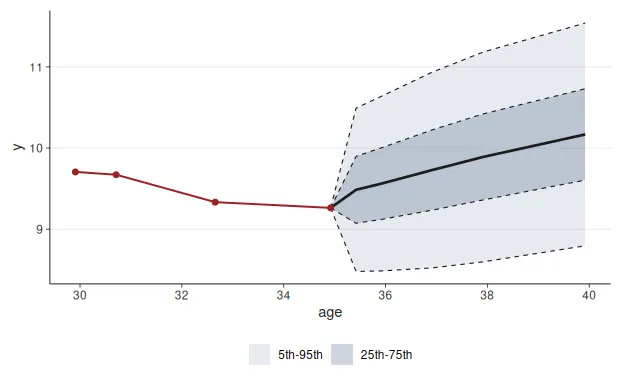
The fan conditions on the fitted process parameters. Its marginal component
uses the same total uncertainty selected by ref_dynamics(), while
kernel_uncertainty = "plug_in" records that uncertainty in the estimated
dependence kernel is not propagated. That omission matters most when repeat
counts or lag coverage are weak.
The forecast distribution obeys every generic of the package: a later
observation can be scored against it with as_scores(), which gives
the same innovation Z that ref_transition() would.
as_scores(fc$dist[2], 10.5)[, c("centile", "z", "tail_prob")]#> # A tibble: 1 × 3#> centile z tail_prob#> <dbl> <dbl> <dbl>#> 1 0.924 1.43 0.152Reading the output
Section titled “Reading the output”components: fractions of normal-score variance that are stable, dynamic, and measurement. A large measurement fraction means visits are noisy and short-interval change is mostly noise; a large stable fraction means people hold their rank and innovation Z is sensitive.r_median_lagwith its SE: the one number the data identify most directly. If the SE is large, do not interpretell.supporton transitions and forecasts:in,extrapolated_lag,unsupported_age,insufficient_history, orunidentified. This records temporal support, not empirical calibration.inferential_statuson transitions distinguishes held-out rows from reused training rows, an unidentified process, and measurement noise that could not be separated.reference_uncertaintyandkernel_uncertaintymake the two uncertainty layers explicit.
PIT-calibrated reference fits are refused by ref_dynamics() for now: the
longitudinal inverse-CDF transformation cannot yet reproduce that map in a
forecast distribution. An adapted reference can be used with crossfit = 0,
but adaptation is refused during cross-fitting because the local map cannot be
re-estimated honestly inside each fold.
Continue with Coming from PCNtoolkit
(vignette("pcntoolkit", package = "referent")), or use
Troubleshooting reference models when the process is
unidentified or a forecast is unsupported.