Brain charts across sites

The standard normative-modelling workflow in neuroimaging is: pool controls from several scanners, estimate the reference distribution of each regional measure as a function of age and sex with a site effect, score every reference subject out of sample, and then score new participants, often from a scanner that contributed no controls. This vignette runs that workflow end to end on a simulated panel and compares four deployment strategies for a new site: the population curve, adaptation, calibration, and a local refit.

library(referent)

A multi-site reference panel

Five sites, with site-specific level shifts and one site with a wider spread. The outcome y plays the role of a regional volume; the three markers are further regions that share a latent factor with y.

ref <- ref_simulate(
  800, sites = 5,
  site_shift = c(0, 0.8, -0.5, 0.3, 0),
  site_log_scale = c(0, 0, 0, 0, 0.2),
  seed = 1
)
ref$participant_id <- sprintf("R%04d", seq_len(nrow(ref)))
regions <- c("y", "marker_01", "marker_02", "marker_03")
table(ref$site)
#>
#>   A   B   C   D   E
#> 152 176 150 157 165

The site effect enters the location as a random effect, s(site, bs = "re"). Unlike a fixed site factor this shrinks small sites toward the pooled curve and, more importantly, gives a well-defined prediction for a level that was not in the reference: the random effect is set to zero and the population curve is used. referent reports those rows with support == "new_group".

spec <- ref_spec(
  family = ref_gaussian(),
  location = ~ s(age, k = 6) + sex + s(site, bs = "re"),
  scale = ~1
)
fit <- ref_fit(spec, data = ref, outcomes = all_of(regions), id = participant_id)
fit
#> <ref_fit> gaussian via mgcv
#> 4 outcomes, n = 800
#> covariates: age, sex, and site
#> status: ok=4
tidy(fit)[, c("outcome", "status", "n", "edf_s(age)", "edf_s(site)")]
#> # A tibble: 4 × 5
#>   outcome   status     n `edf_s(age)` `edf_s(site)`
#>   <chr>     <chr>  <int>        <dbl>         <dbl>
#> 1 y         ok       800         2.73      3.78
#> 2 marker_01 ok       800         1.59      0.000287
#> 3 marker_02 ok       800         1.00      0.00114
#> 4 marker_03 ok       800         2.24      1.99

autoplot(fit, type = "centiles", outcome = "y", by = sex)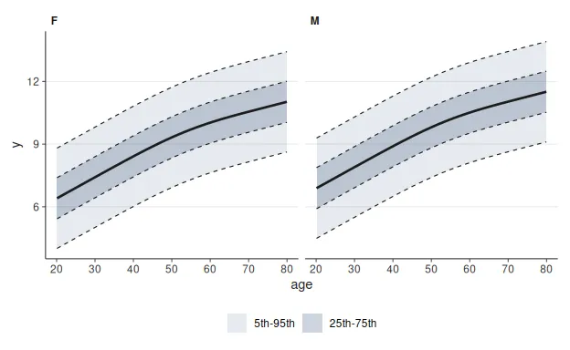

Scaling to many outcomes

A regional panel has tens of outcomes; a vertex-wise or voxel-wise chart has tens of thousands. ref_fit() fits each outcome independently, so the problem is embarrassingly parallel, and the package has three levers for it.

Parallel fits in one session. When future.apply is installed and a non-sequential plan is active, outcomes are fitted across workers. Nothing else changes: the same call, the same object back.

future::plan(future::multisession, workers = 8)
fit_wide <- ref_fit(spec, data = wide, outcomes = starts_with("vertex_"))
future::plan(future::sequential)

Memory per outcome, and why to freeze. Each fitted outcome carries its mgcv model, including the model frame, fitted values, and residuals; those are what make a fit large. ref_freeze() keeps only what prediction needs (coefficients, their covariance, the smooth constructions, factor levels) and reproduces the fit’s predictions exactly. On 20 outcomes at n = 5000, the fit is about 14 MB and the bundle about 3 MB, a factor of 4.6; the saving grows with n because the bundle’s size does not depend on it.

wide <- ref_simulate(5000, seed = 1)
set.seed(2)
for (j in 1:20) wide[[sprintf("vertex_%02d", j)]] <- wide$y + rnorm(5000)
wide_spec <- ref_spec(ref_gaussian(), ~ s(age, k = 6) + sex, scale = ~1)
fit_wide <- ref_fit(wide_spec, wide, outcomes = starts_with("vertex_"))
bundle_wide <- ref_freeze(fit_wide)
c(fit = format(object.size(fit_wide), units = "MB"),
  bundle = format(object.size(bundle_wide), units = "MB"))
#>       fit    bundle
#> "13.7 Mb"  "2.9 Mb"

Blocks as independent jobs. For a matrix too wide to hold in one session, split the outcome columns into blocks, fit each block as its own job, and combine the score tables afterwards. Outcomes share no state in ref_fit(), so the combined result is identical to one big fit. The demo below fits 12 outcomes as three blocks of four and checks that claim.

vertices <- sprintf("vertex_%02d", 1:12)
target <- ref_simulate(50, seed = 3)
for (v in vertices) target[[v]] <- target$y + rnorm(50)
single <- ref_fit(wide_spec, wide, outcomes = all_of(vertices))
blocks <- split(vertices, rep(1:3, each = 4))
block_fits <- lapply(blocks, function(b) ref_fit(wide_spec, wide, outcomes = all_of(b)))

z_single <- predict(single, target, uncertainty = "conditional")
z_blocks <- vctrs::vec_rbind(!!!lapply(block_fits, predict, newdata = target,
                                       uncertainty = "conditional"))
identical(z_single$z, z_blocks$z)
#> [1] TRUE

The same holds for augment(): the wide per-observation frames from each block share the covariate columns and can be joined on .row. On a cluster, the block is the array index. A fit_block.R that reads its block of columns, fits, freezes, and saves the bundle is the whole job:

# fit_block.R, run as: Rscript fit_block.R $SLURM_ARRAY_TASK_ID
block <- as.integer(commandArgs(trailingOnly = TRUE)[[1]])
columns <- readRDS("outcome_blocks.rds")[[block]]   # list of column-name vectors
wide <- arrow::read_parquet("reference.parquet", col_select = c("age", "sex", "site", columns))
fit <- ref_fit(spec, wide, outcomes = all_of(columns))
ref_write(ref_freeze(fit), sprintf("bundles/block_%04d.rds", block))

#SBATCH --array=1-100
#SBATCH --cpus-per-task=1 --mem=4G
Rscript fit_block.R $SLURM_ARRAY_TASK_ID

Scoring a new cohort is then vctrs::vec_rbind() over predict(ref_read(path, trusted = TRUE), newdata) for each trusted bundle. Because bundles are small, the 100 of them for 100k vertices are a few hundred megabytes, and scoring reads them one at a time.

Out-of-fold reference scores

Scoring the reference rows with the model that was fit to them understates their deviations. ref_crossfit() gives every reference row a score from a fold that excluded it, stratified by site so that each fold’s model still sees every scanner. These scores are the honest reference for anything downstream: calibration checks, the joint model, and the expected exceedance rate.

cf <- ref_crossfit(spec, data = ref, outcomes = all_of(regions), folds = 5,
                    strata = site, id = participant_id)
oof <- split(cf, cf$.outcome)
oof_calibration <- data.frame(
  region = names(oof),
  n = sapply(oof, nrow),
  n_scored = sapply(oof, function(s) sum(is.finite(s$z))),
  mean_z = round(sapply(oof, function(s) mean(s$z, na.rm = TRUE)), 3),
  var_z = round(sapply(oof, function(s) var(s$z, na.rm = TRUE)), 3),
  cover_95 = round(sapply(oof, function(s) mean(abs(s$z) < qnorm(0.975), na.rm = TRUE)), 3),
  crps = round(sapply(oof, function(s) mean(s$crps, na.rm = TRUE)), 3),
  row.names = NULL
)
oof_calibration
#>      region   n n_scored mean_z var_z cover_95  crps
#> 1 marker_01 800      796  0.004 1.008    0.935 0.648
#> 2 marker_02 800      796  0.001 1.016    0.956 0.664
#> 3 marker_03 800      796  0.002 1.022    0.940 0.609
#> 4         y 800      796  0.005 1.021    0.947 0.827

A few rows have no out-of-fold z: their age lies outside the range of the fold that scored them, so support is "out" and z is masked. That is the extrapolation rule doing its job, not a failure.

Scoring a new site

A sixth scanner arrives with 200 participants. Its level differs from every reference site. Thirty of its participants are known controls; the rest are the people we want to score.

new_site <- ref_simulate(
  1500, sites = 6,
  site_shift = c(0, 0.8, -0.5, 0.3, 0, 1.0),
  site_log_scale = c(0, 0, 0, 0, 0.2, 0),
  seed = 2
)
new_site <- new_site[new_site$site == "F", ][1:200, ]
new_site$participant_id <- sprintf("F%04d", seq_len(nrow(new_site)))
controls <- new_site[1:30, ]
held_out <- new_site[31:200, ]
table(ref_support(fit, held_out)$support)
#>
#> new_group
#>       170

There are four options, and they answer different questions.

1. Score against the population curve. Use the fit as it is. The random effect for site F is zero, so the scores are relative to the average reference site. Any level difference of the scanner becomes a shift in everyone’s z.
2. Adapt. ref_adapt() freezes the shared trajectory and estimates a shrunk location (and optionally scale) offset for site F from the 30 controls. This is the right tool when the scanner moves the measurements but the age trend is shared.
3. Calibrate by site. ref_calibrate(by = site) re-maps the PIT values of site F through their empirical distribution on the 30 controls. It fixes probabilities rather than parameters and needs more local data to do so without noise.
4. Refit with the 30 controls appended and site F as a sixth level. This is the most flexible but the least stable with few controls, and it changes the reference for everyone else.

adapted <- ref_adapt(fit, data = controls, by = site,
                      parameters = c("location", "scale"))
calibrated <- ref_calibrate(fit, data = controls, by = site)
refit <- ref_fit(spec, data = rbind(ref, controls), outcomes = all_of(regions),
                  id = participant_id)
adapted$adaptation
#> <ref_adaptation> parameters: location, scale
#> local n = 30
#> y / F: location 1.28, scale x0.981 (n = 30)
#> marker_01 / F: location 0.313, scale x0.951 (n = 30)
#> marker_02 / F: location 0.139, scale x0.9 (n = 30)
#> marker_03 / F: location 0.0358, scale x0.999 (n = 30)

The first three objects still record site F as support == "new_group" because the original reference contained no site-F rows. Adaptation or calibration estimates a transport map; it does not rewrite that provenance. The calls below therefore set allow_extrapolation = TRUE deliberately after estimating the map from known controls. Without that explicit opt-in, referent masks the scores.

Each strategy is judged on the 170 held-out site-F rows. Because site F was simulated from the same generator as the reference, a correct strategy must return calibrated scores there: mean_z near 0, var_z near 1, 95% coverage near 0.95. Thirty controls bound what any local strategy can achieve: the standard error of a 30-person mean z is about 0.18, and the controls themselves sit where chance put them relative to the rest of site F.

ctrl_scores <- predict(fit, newdata = controls, type = "scores", outcomes = "y",
                       allow_extrapolation = TRUE)
c(controls_mean_z = round(mean(ctrl_scores$z), 2),
  held_out_mean_z = round(mean(predict(fit, newdata = held_out, type = "scores",
                                       outcomes = "y",
                                       allow_extrapolation = TRUE)$z), 2))
#> controls_mean_z held_out_mean_z
#>            1.15            0.73

strategies <- list(population = fit, adapted = adapted, calibrated = calibrated, refit = refit)
strategy_scores <- lapply(strategies, function(model) {
  predict(model, newdata = held_out, type = "scores", outcomes = "y",
          allow_extrapolation = TRUE)
})
comparison <- do.call(rbind, lapply(names(strategy_scores), function(nm) {
  sc <- strategy_scores[[nm]]
  ok <- is.finite(sc$z) & is.finite(sc$log_density)
  data.frame(
    strategy = nm,
    mean_z = round(mean(sc$z[ok]), 2),
    var_z = round(var(sc$z[ok]), 2),
    cover_95 = round(mean(sc$centile[ok] > 0.025 & sc$centile[ok] < 0.975), 3),
    log_score = round(mean(sc$log_density[ok]), 3)
  )
}))
comparison
#>     strategy mean_z var_z cover_95 log_score
#> 1 population   0.73  0.83    0.906    -1.991
#> 2    adapted  -0.13  0.84    0.976    -1.731
#> 3 calibrated  -0.46  0.96    0.941    -1.821
#> 4      refit  -0.32  0.83    0.965    -1.775

The population-curve scores carry the scanner’s level shift into mean_z and pay for it in log score. The three local strategies remove most of the shift, and what remains is the difference between the 30 controls and the other 170 participants, which none of them can know. They differ in how they spend the 30 observations. Adaptation estimates two numbers (a shrunk location and log-scale offset) on the family’s own likelihood and leaves the age curve alone, so it is the most stable. Calibration by site re-maps probabilities through a four-parameter sinh-arcsinh map on the normal scores; its centre is as good as the controls’ mean, but its spread and tail parameters are noisy at this sample size. The refit lets the controls move the shared smooth and the random-effect variance as well as the site level, and it changes the reference for every other site. In this simulation with 30 controls, adaptation spends the local information on two parameters and is more stable than the rank map or refit. That is an illustration, not a general sample-size rule: choose and validate a transport strategy with held-out local controls whenever the design permits it.

autoplot(adapted, type = "adaptation")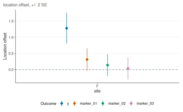

Joint deviation across regions

Per-region Z-scores are correlated; a participant who is low on every region is more unusual than four independent z = -1.5 values suggest. ref_joint() fits a Gaussian copula on the out-of-fold reference scores, with a shrinkage correlation estimate, and returns a joint centile calibrated through the reference distribution of the Mahalanobis statistic. Missing regions are handled by the observed submatrix.

joint <- ref_joint(cf)
joint
#> <ref_joint> gaussian copula, 4 outcomes, n = 796 reference subjects
#> shrinkage lambda = 0.00611
new_scores <- predict(adapted, newdata = held_out, type = "scores",
                      allow_extrapolation = TRUE)
joint_scores <- predict(joint, new_scores)
head(joint_scores)
#> # A tibble: 6 × 7
#>    .row .id      d2 n_observed base_centile joint_centile  joint_z
#>   <int> <chr> <dbl>      <dbl>        <dbl>         <dbl>    <dbl>
#> 1     1 F0031  5.42          4        0.753         0.731  0.615
#> 2     2 F0032  4.91          4        0.703         0.696  0.512
#> 3     3 F0033  5.60          4        0.769         0.747  0.666
#> 4     4 F0034  1.88          4        0.241         0.248 -0.681
#> 5     5 F0035  3.32          4        0.494         0.497 -0.00629
#> 6     6 F0036  2.18          4        0.298         0.307 -0.505
mean(joint_scores$joint_centile > 0.95, na.rm = TRUE)
#> [1] 0.04117647

Flags, and how many to expect

ref_flag() marks |z| > 2 per region and adds FDR-adjusted two-sided tail probabilities across all region-by-person tests. Under calibration about 4.6% of rows exceed the threshold by chance; the attribute expected_exceedances is that count.

flags <- ref_flag(new_scores, threshold = 2)
c(observed = attr(flags, "observed_exceedances"),
  expected = round(attr(flags, "expected_exceedances"), 1))
#> observed expected
#>     29.0     30.9
sum(flags$fdr < 0.05, na.rm = TRUE)
#> [1] 0

autoplot(new_scores[new_scores$.row <= 15, ], type = "heatmap")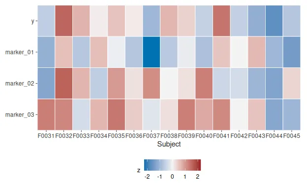

What to report

• The reference: ref_freeze(fit) prints a model card with the family, formulas, covariate ranges, site levels, and software versions. Ship the frozen bundle, not the training data.
• Out-of-fold calibration of the reference (the oof_calibration table), which is the evidence that the scores mean what they claim.
• For each new site: how it was scored (population, adapted, calibrated, or refit), the number of local controls, the estimated offsets with their standard errors, and the held-out calibration if any controls were held back.
• The expected and observed exceedance counts, and the joint centiles, rather than a list of flagged people.

ref_freeze(adapted, criteria = "healthy controls, 20-80 years", units = "mm^3")
#>
#> ── referent model card ─────────────────────────────────────────────────────────
#> bundle schema: 1.0.0
#> family: gaussian
#> engine: mgcv
#> outcomes: y, marker_01, marker_02, and marker_03
#> covariates: age, sex, and site
#> n: 800
#> missing-data policy: complete-case per outcome; predictors are never imputed
#> package 0.1.0, mgcv 1.9.4, R 4.6.1
#> statuses: y=ok, marker_01=ok, marker_02=ok, marker_03=ok
#> adapted: location, scale (local n = 30)
#> Covariate ranges
#> age: [20.11, 79.97]

Ship and reuse a reference

A reference is useful to other sites only if it can be applied without the training data. ref_freeze() produces that object; ref_write() persists it.

bundle <- ref_freeze(fit, criteria = "healthy controls, 20-80 years", units = "mm^3")
bundle_path <- file.path(tempdir(), "reference-v1.rds")
ref_write(bundle, bundle_path)
file.size(bundle_path)
#> [1] 31408

The bundle contains, per outcome, the coefficients, their covariance Vp, the smooth bases, the terms and factor levels (xlevels), plus the support reference (covariate ranges and factor levels), the calibration and adaptation slots if any were estimated, the reference-sample baseline used by standardized_log_score, and the model card. It excludes the training rows, the model frame, fitted values, and residuals. That reduces direct disclosure, but it is not a privacy guarantee: coefficients and retained factor levels can still reveal information about small or unique groups. Treat a bundle as a sensitive model artifact, review it under the same disclosure policy as other fitted models, and do not describe it as anonymised or differentially private. RDS is also executable R serialization, so accept bundles only from an authenticated, trusted source and verify their provenance through an independent channel.

A receiving site needs only the file and the package. Everything that applies to a ref_fit applies to the bundle: scoring, support checks, adaptation, and calibration.

reference <- ref_read(bundle_path, trusted = TRUE)
reference
#>
#> ── referent model card ─────────────────────────────────────────────────────────
#> bundle schema: 1.0.0
#> family: gaussian
#> engine: mgcv
#> outcomes: y, marker_01, marker_02, and marker_03
#> covariates: age, sex, and site
#> n: 800
#> missing-data policy: complete-case per outcome; predictors are never imputed
#> package 0.1.0, mgcv 1.9.4, R 4.6.1
#> statuses: y=ok, marker_01=ok, marker_02=ok, marker_03=ok
#> Covariate ranges
#> age: [20.11, 79.97]
local_scores <- predict(reference, newdata = held_out, outcomes = "y",
                        allow_extrapolation = TRUE)
table(ref_support(reference, held_out)$support)
#>
#> new_group
#>       170
local_adapted <- ref_adapt(reference, data = controls, by = site)
local_calibrated <- ref_calibrate(reference, data = controls, by = site)
local_adapted$adaptation
#> <ref_adaptation> parameters: location
#> local n = 30
#> y / F: location 1.28, scale x1 (n = 30)
#> marker_01 / F: location 0.313, scale x1 (n = 30)
#> marker_02 / F: location 0.139, scale x1 (n = 30)
#> marker_03 / F: location 0.0358, scale x1 (n = 30)

The bundle’s predictions are the fit’s predictions, not an approximation:

identical(
  predict(fit, held_out, outcomes = "y", uncertainty = "conditional",
          allow_extrapolation = TRUE)$z,
  predict(reference, held_out, outcomes = "y", uncertainty = "conditional",
          allow_extrapolation = TRUE)$z
)
#> [1] TRUE

Versioning. The printed card records the package, mgcv, and R versions that produced the bundle. bundle$data_hash is a SHA-256 digest of the R-serialized training frame used by the fit: included columns are sorted and row names are removed, while values and row order are retained. It binds a bundle to that exact R-side input without storing the frame, but R serialization is not a cross-language canonical data format. If interoperable provenance is required, define and retain a separate canonical file or table digest in the release receipt. Name files by reference version (reference-v1.rds), not by date, and treat a change in the reference cohort, the specification, or the package major version as a new reference: scores from different references are not comparable, and the fingerprint is how a reader can tell two bundles apart.

bundle$versions
#> $referent
#> [1] "0.1.0"
#>
#> $mgcv
#> [1] "1.9.4"
#>
#> $r
#> [1] "4.6.1"
bundle$data_hash
#> [1] "70f933d0cd5c882456183fc043bc8e81ee9d01c67b9fc2f773478de896242039"

Continue with Longitudinal change (vignette("longitudinal-change", package = "referent")), or use Troubleshooting reference models when transported scores remain masked or unstable.