Smoothing and filtering • neuroim2

library(neuroim2)

Filtering trades detail for noise. neuroim2 offers six filters that make the trade differently: some blur everything, some try to keep edges, one sharpens instead, and two work across time as well as space. This article shows what each does to the same image, measured rather than asserted.

anat <- demo_anatomy()
brain <- demo_anatomy_mask()

spacing(anat)
#> [1] 1 1 1

That 1 mm matters for everything below: kernel widths are specified in millimetres, so what a filter actually does depends on sigma relative to the voxel size. On this image the two happen to coincide.

Every number in this article is computed inside the brain mask. Statistics over the whole array are dominated by the 75% of voxels that are air, where every filter looks identical and every difference is invisible.

inside <- which(as.vector(brain))
baseline <- as.array(anat)[inside]

A helper to compare slices on a shared intensity scale:

compare <- function(..., z = 24) {
  imgs <- list(...)
  zlim <- range(vapply(imgs, function(v) range(v[, , z]), numeric(2)))
  op <- par(mfrow = c(1, length(imgs)), mar = c(0.5, 0.5, 2, 0.5))
  for (nm in names(imgs)) {
    image(imgs[[nm]][, , z],
      main = nm, zlim = zlim, col = gray.colors(256), axes = FALSE, asp = 1
    )
  }
  par(op)
}

Gaussian blur

gaussian_blur() is the fast, unconditional baseline: every voxel becomes a weighted average of its neighbours regardless of what is there.

light <- gaussian_blur(anat, brain, fwhm = 4)
heavy <- gaussian_blur(anat, brain, fwhm = 9)

compare(original = anat, `FWHM 4 mm` = light, `FWHM 9 mm` = heavy)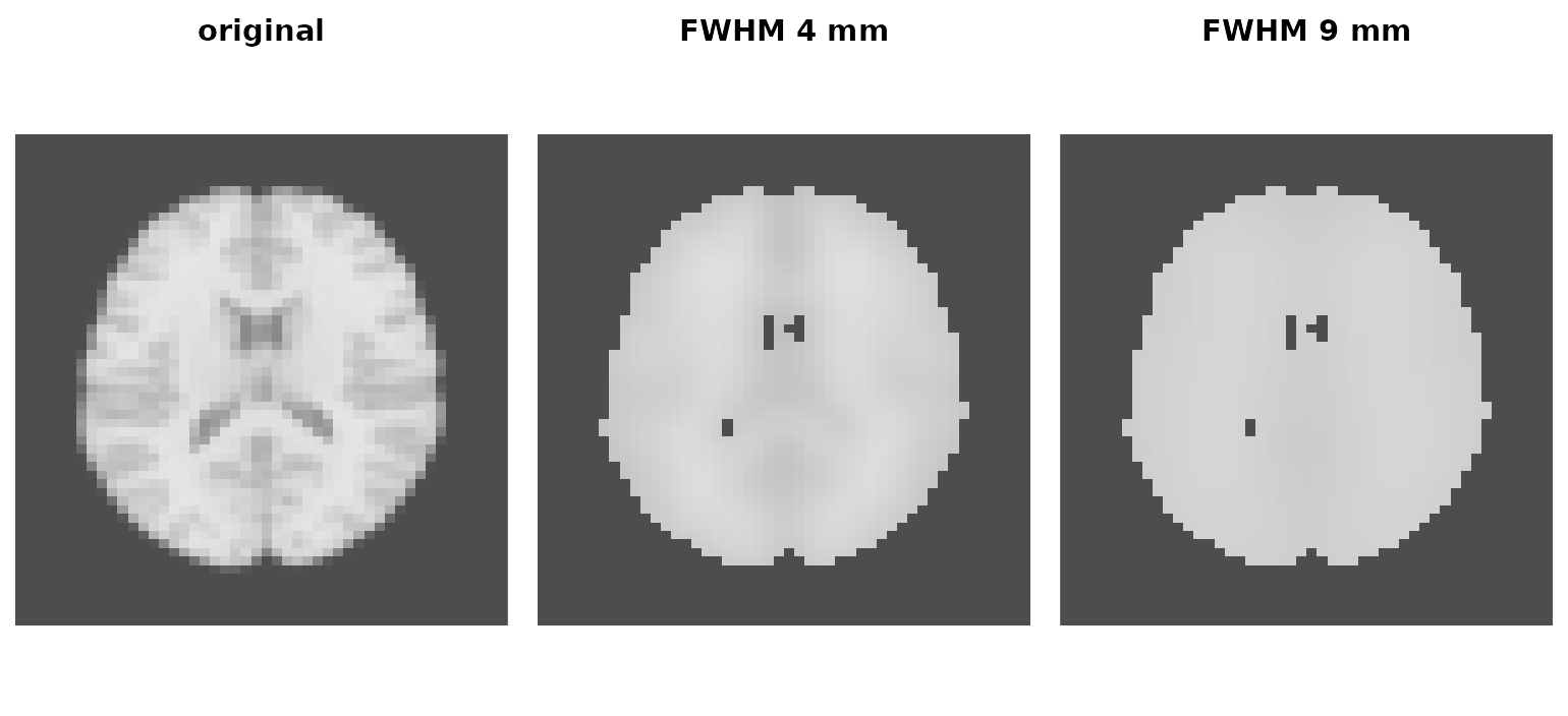

Three axial slices: original, lightly smoothed, heavily smoothed.

Gaussian smoothing at two kernel widths.

Specify the width however you like: fwhm in millimetres, which is the unit smoothing is usually reported in, or sigma in millimetres, which is the same thing divided by 2 * sqrt(2 * log(2)). Either way the kernel is sized from what you asked for, so the smoothing you get is the smoothing you specified:

# The point-spread function is the operator: smooth an impulse, read the width
# back out. This is the only honest check that a request was honoured.
psf_fwhm <- function(v, sp) {
  a <- as.array(v); a[a < 0] <- 0
  prof <- apply(a, 1, sum); off <- (seq_along(prof) - 21) * sp
  mu <- sum(prof * off) / sum(prof)
  2 * sqrt(2 * log(2)) * sqrt(sum(prof * (off - mu)^2) / sum(prof))
}
imp_sp <- NeuroSpace(c(41L, 41L, 41L), c(2, 2, 2))
imp <- array(0, c(41, 41, 41)); imp[21, 21, 21] <- 1
imp <- NeuroVol(imp, imp_sp)

c(
  `asked 4 mm` = psf_fwhm(gaussian_blur(imp, fwhm = 4, normalize = FALSE), 2),
  `asked 9 mm` = psf_fwhm(gaussian_blur(imp, fwhm = 9, normalize = FALSE), 2)
)
#> asked 4 mm asked 9 mm 
#>   3.999316   8.999333

window is still there, and still means what it always did: the kernel support in voxels either side, which truncates the Gaussian. Passing it reproduces the old behaviour exactly, and that behaviour is worth seeing, because it is easy to under-smooth by a lot without noticing:

c(
  `sigma 4, window 1` = psf_fwhm(gaussian_blur(imp, sigma = 4, window = 1, normalize = FALSE), 2),
  `sigma 4, window 2` = psf_fwhm(gaussian_blur(imp, sigma = 4, window = 2, normalize = FALSE), 2),
  `sigma 4, derived`  = psf_fwhm(gaussian_blur(imp, sigma = 4, normalize = FALSE), 2),
  `requested`         = 2 * sqrt(2 * log(2)) * 4
)
#> sigma 4, window 1 sigma 4, window 2  sigma 4, derived         requested 
#>          3.762809          6.074223          9.417647          9.419280

A sigma of 4 mm inside window = 1 delivers under 4 mm FWHM where 9.4 mm was asked for, and because window counts voxels while sigma is in millimetres, the shortfall depends on the voxel size — the same call smooths a 1 mm structural and a 3 mm EPI differently. Leave window alone unless you have a specific reason to clip the kernel; truncate (default 4 standard deviations) is the knob for trading accuracy against speed.

Handing gaussian_blur() a NeuroVec smooths every volume with the same kernel, and does it in one compiled call over the whole run rather than a loop in R — so pass the run, do not loop over x[[i]] yourself. Volumes are smoothed in parallel; RcppParallel::setThreadOptions() sets how many at a time.

Edge-preserving filters

Gaussian blur does not know where anatomy stops. guided_filter() fits local linear models, smoothing within regions and leaving boundaries alone. bilateral_filter() weights neighbours by intensity similarity as well as distance, so voxels across a tissue boundary contribute little.

One parameter needs care. bilateral_filter()’s intensity_sigma is a multiple of the image’s own standard deviation, but guided_filter()’s epsilon is absolute, in squared intensity units. On an image scaled 0 to 9533 an epsilon of 0.5 is indistinguishable from zero; it has to be scaled to the data.

sd_in <- sd(baseline)

guided <- guided_filter(anat, radius = 1, epsilon = (0.6 * sd_in)^2)
bilateral <- bilateral_filter(anat, brain, spatial_sigma = 2, intensity_sigma = 1, window = 1)

compare(original = anat, gaussian = light, guided = guided, bilateral = bilateral)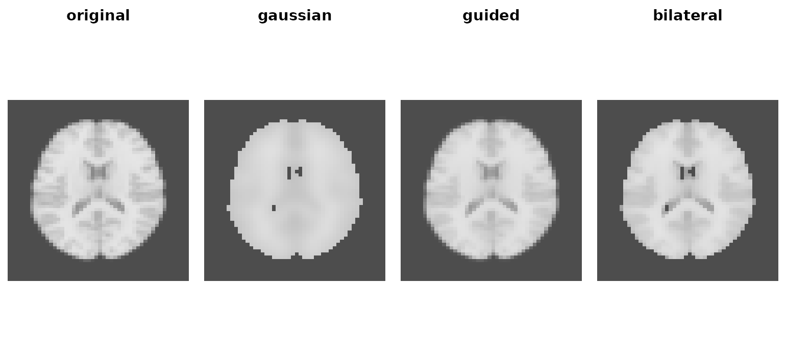

Four axial slices comparing original, Gaussian, guided and bilateral filtering.

Gaussian blur against two edge-preserving filters at matched support.

All three now use a one-voxel radius, so the comparison is about method rather than support. The question an edge-preserving filter has to answer is: how much variance can you remove per unit of distortion?

score <- function(x) {
  v <- as.array(x)[inside]
  removed <- 1 - var(v) / var(baseline)
  distortion <- 1 - cor(v, baseline)
  c(sd = sd(v), removed = removed, distortion = distortion,
    ratio = removed / distortion)
}

round(rbind(
  original = score(anat),
  gaussian = score(light),
  guided = score(guided),
  bilateral = score(bilateral)
), 3)
#>                 sd removed distortion  ratio
#> original  1350.807   0.000      0.000    NaN
#> gaussian   556.862   0.830      0.283  2.933
#> guided    1291.002   0.087      0.027  3.231
#> bilateral 1080.282   0.360      0.029 12.294

bilateral_filter() removes a third of the variance for a twentieth of the distortion — an exchange rate three times better than the Gaussian’s, and that ratio is what “edge preserving” buys you. gaussian_blur() removes more variance outright but pays the most per unit for it. guided_filter() is the weakest of the three at this epsilon: it barely smooths, and the little it does costs about what the Gaussian charges. Raise epsilon towards sd_in^2 to get more out of it.

Note that a plain whole-array sd() would have told you the opposite story. Outside the mask these images are nearly constant, so filters that flatten air look like strong denoisers when scored over the full volume.

Sharpening

laplace_enhance() runs the other way, amplifying detail with a multi-scale non-local scheme. It is a display and detection aid, not a denoiser.

sharp <- laplace_enhance(anat, brain, k = 2, patch_size = 3, search_radius = 1, h = 0.7)

compare(original = anat, enhanced = sharp)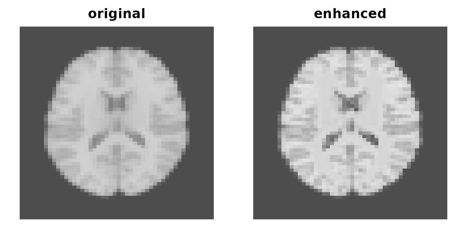

Two axial slices: original and sharpened.

Laplacian enhancement increases local contrast rather than reducing it.

Pass the mask, whose second argument position is easy to skip. It is what keeps the enhancement off the background — and the background is where over-enhancement shows first:

outside <- which(as.vector(brain) == 0)
sharp_arr <- as.array(sharp)

round(rbind(
  original = c(inside = sd(baseline), outside = sd(as.array(anat)[outside])),
  enhanced = c(sd(sharp_arr[inside]), sd(sharp_arr[outside]))
), 2)
#>           inside outside
#> original 1350.81  269.99
#> enhanced 2133.71  269.99

Contrast inside the brain rises by more than half, which is the point, and the noise floor outside is untouched because the mask excluded it. Drop the mask and that second column climbs instead.

The output does go negative on a non-negative image, so clip before writing anything downstream:

range(sharp_arr)
#> [1]  -122.0209 11914.8799

Filtering across time

Two filters work on a NeuroVec, over space and time together. Both need a series with real temporal structure:

bold_mask <- demo_mask()
bold <- demo_bold(n_time = 40)

attr(bold, "TR")
#> [1] 2

bilateral_filter_4d() extends the bilateral idea along the time axis. temporal_spacing is the units of that axis, so it must be your TR — here read straight off the simulated series rather than assumed:

bf4d <- bilateral_filter_4d(
  bold, bold_mask,
  spatial_sigma = 4, intensity_sigma = 1, temporal_sigma = 1,
  spatial_window = 1, temporal_window = 1,
  temporal_spacing = attr(bold, "TR")
)

cgb_filter() decides which voxels belong together by correlating their time courses rather than comparing intensities. It builds a sparse graph — spatial proximity times time-series affinity — and diffuses over it, which is the right model for functional data where two voxels in a network should smooth together even if their raw intensities differ.

out <- cgb_filter(
  bold, mask = bold_mask,
  spatial_sigma = 5, window = 1,
  corr_map = "power", corr_param = 2,
  topk = 16, passes = 1, lambda = 1,
  return_graph = TRUE
)

Both should reduce per-voxel noise. Measure on a random sample of in-mask voxels — taking the first 300 by linear index gives you a contiguous patch in the bottom slice, where support is truncated and neighbours are trivially correlated:

set.seed(1)
sample_idx <- sample(which(as.vector(bold_mask) > 0), 300)

noise <- function(x) mean(apply(as.matrix(x)[sample_idx, ], 1, sd))

c(raw = noise(bold), bilateral_4d = noise(bf4d), cgb = noise(out$result))
#>          raw bilateral_4d          cgb 
#>    1.1665227    0.8299609    0.7860965

return_graph = TRUE kept the graph, so further passes cost nothing to set up:

c(
  raw = noise(bold),
  pass_1 = noise(out$result),
  pass_2 = noise(cgb_smooth(bold, out$graph, passes = 2))
)
#>       raw    pass_1    pass_2 
#> 1.1665227 0.7860965 0.6383422

Building the graph is the expensive part of cgb_filter(); cgb_smooth() reuses it, which is how you explore passes and lambda without paying for it each time.

Choosing

Want	Use	Watch out for
A fast, predictable baseline	`gaussian_blur()`	give `fwhm` or `sigma`; setting `window` truncates the kernel
Denoise but keep boundaries	`bilateral_filter()`	`intensity_sigma` scales with the image SD
Same, local-linear formulation	`guided_filter()`	`epsilon` is absolute, in intensity squared
More visible detail, not less	`laplace_enhance()`	raises the noise floor; can go negative
Joint space and time denoising	`bilateral_filter_4d()`	`temporal_spacing` must be your TR
Smoothing that follows networks	`cgb_filter()`	needs real temporal structure

Where to go next

vignette("visualization") — inspecting the results of any of these
vignette("resampling-and-orientation") — changing the grid rather than the values
?gaussian_blur, ?guided_filter, ?cgb_filter, ?cgb_smooth