Resampling and orientation
Source:vignettes/resampling-and-orientation.Rmd
resampling-and-orientation.RmdResampling changes the grid on which an image is represented. Reorientation changes the order and direction of its axes. Both can change array dimensions, but they handle voxel values differently:
| Operation | Handles voxel values by | Preserves anatomy in world space | Use when |
|---|---|---|---|
downsample() |
averaging into coarser bins | yes | you want fewer voxels |
resample_to() |
interpolating onto a target grid | yes, within the target field of view | you must match another image |
as_canonical() |
permuting and flipping exactly | yes | you want RAS array orientation |
deoblique() |
interpolating onto an axis-aligned grid | yes | the affine is oblique |
reorient() operates on a NeuroSpace,
returning the geometry for a permuted and flipped grid. Use
as_canonical() on an image to update its array and space
together. Replacing only the space on an unchanged array assigns values
to the wrong world positions.
anat <- demo_anatomy()
mask <- demo_mask()
Downsampling
downsample() keeps the field of view and coarsens the
grid. Give it exactly one of factor, spacing
or outdim:
half <- downsample(anat, factor = 0.5)

dim(anat)
#> [1] 48 57 48
dim(half)
#> [1] 24 28 24
round(spacing(half), 3)
#> [1] 8.042 8.179 8.042
The result is no longer isotropic, because
round(57 * 0.5) is 28 rather than 28.5 — rounding a grid
always perturbs the spacing slightly.
op <- par(mfrow = c(1, 2), mar = c(1, 1, 2, 1))
image(seq_len(dim(anat)[1]), seq_len(dim(anat)[2]), anat[, , 24],
  main = "original", col = gray.colors(256), axes = FALSE, ann = TRUE,
  xlab = "", ylab = "", asp = 1
)
image(seq(1, dim(anat)[1], length.out = dim(half)[1]),
  seq(1, dim(anat)[2], length.out = dim(half)[2]), half[, , 12],
  main = "factor = 0.5", col = gray.colors(256), axes = FALSE, ann = TRUE,
  xlab = "", ylab = "", asp = 1
)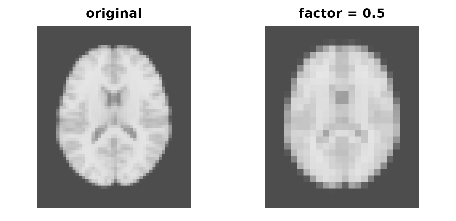
Full and half resolution, drawn at matched physical extent.
par(op)downsample() box-averages, which is right for intensity
images and wrong for labels — averaging label 3 and label 5 gives you
label 4.
Resampling onto a target grid
resample_to() puts an image onto any grid you name.
Building that grid is where things go wrong, so start there.
Build the target from the source affine
It is tempting to describe a target with dim,
spacing and origin. Do not: those three do not
carry orientation, and the constructor produces an
axis-aligned RAS affine regardless of what the source looked like.
affine_to_axcodes(trans(mask))
#> [1] "L" "A" "S"

naive <- NeuroSpace(round(dim(mask) * 1.6), spacing(mask) / 1.6, origin = origin(mask))
affine_to_axcodes(trans(naive))
#> [1] "R" "A" "S"
The source runs LAS and the target runs
RAS. The target’s first axis points in the opposite
direction from the same origin, placing its grid where the source has no
data. Resampling into it warns about the lack of overlap and returns an
empty image:
sum(resample_to(mask, naive, method = "nearest"))
#> Warning: The resample target covers little of the source image.
#> ! Their world bounding boxes overlap over 0% of the target, so most of the
#>   output will be background.
#> ℹ Source spans [-108.5, 112.0] [-108.5, 112.0] [-46.2, 42.6] and the target
#>   [112.0, 332.9] [-108.5, 112.4] [-46.2, 43.9].
#> ℹ A target built with `NeuroSpace(dim, spacing, origin)` gets a
#>   positive-diagonal affine, which mirrors a source whose x axis runs the other
#>   way. Pass `trans =` explicitly, or use `resample_to()` with the image you
#>   want to match.
#> [1] 0
Scale the source’s own affine instead, which keeps orientation and origin intact:
tr <- trans(mask)
tr[1:3, 1:3] <- tr[1:3, 1:3] / 1.6

finer <- NeuroSpace(round(dim(mask) * 1.6), trans = tr)

affine_to_axcodes(trans(finer))
#> [1] "L" "A" "S"
round(spacing(finer), 3)
#> [1] 2.188 2.188 2.312
Then check the result, every time. The affine was scaled by 1.6 in
each direction, so each new voxel has 1 / 1.6^3 of the
original voxel volume. Compare physical mask volumes:
up <- resample_to(mask, finer, method = "nearest")

source_mm3 <- sum(mask) * prod(spacing(mask))
resampled_mm3 <- sum(up) * prod(spacing(up))
c(source_mm3 = source_mm3, resampled_mm3 = resampled_mm3)
#>    source_mm3 resampled_mm3
#>       1338538       1329275

abs(resampled_mm3 / source_mm3 - 1)
#> [1] 0.006920062
Small differences are expected from nearest-neighbour boundary sampling. Larger differences warrant checking the target field of view and resolution; rounding target dimensions can also change its physical extent.
Choosing an interpolation method
"nearest", "linear" and
"cubic" are available and the default is
"nearest", so pass "linear" explicitly for
continuous data. The rule is labels and masks take
"nearest", continuous data takes "linear" or
"cubic", and the reason is one number:
lin <- resample_to(mask, finer, method = "linear")
a <- as.array(lin)

fractional <- sum(abs(a - round(a)) > 1e-6)
c(voxels = fractional, of_resampled_mask = fractional / sum(up))
#>            voxels of_resampled_mask
#>      2.283700e+04      1.901087e-01
Nearly a fifth of the mask comes back as values strictly between 0 and 1. Those voxels are neither in nor out, and every count taken afterwards is wrong.
Nearest is not free either: it preserves the label set, not
the volume. Any mask resample changes how many voxels are in
the mask, so check sum() whichever method you use.
Matching another image
The common real task needs no target construction — pass the image whose grid you want:
coarse <- downsample(mask, factor = 0.5) # used only as a grid donor
matched <- resample_to(mask, coarse, method = "nearest")

identical(dim(matched), dim(coarse))
#> [1] TRUE
identical(trans(space(matched)), trans(space(coarse)))
#> [1] TRUE
Two images that share a NeuroSpace can be compared,
overlaid and subtracted. Two that do not, cannot — several plotting
helpers require it explicitly rather than resampling silently behind
your back.
Reorienting
reorient() rewrites a space so its axes carry different
codes, without touching a single voxel.
vignette("spaces-and-coordinates") covers the codes
themselves; what matters here is what it does to positions.
ras <- reorient(space(mask), c("R", "A", "S"))

affine_to_axcodes(trans(space(mask)))
#> [1] "L" "A" "S"
affine_to_axcodes(trans(ras))
#> [1] "R" "A" "S"
The same numerical grid index can now refer to a different world position:
rbind(
  before = as.vector(grid_to_coord(space(mask), matrix(c(1, 1, 1), nrow = 1))),
  after = as.vector(grid_to_coord(ras, matrix(c(1, 1, 1), nrow = 1)))
)
#>          [,1]   [,2]   [,3]
#> before  112.0 -108.5 -46.25
#> after  -108.5 -108.5 -46.25
That compares two grid corners, not the position of the same
anatomical voxel. There is no reorient() method for a
NeuroVol. To reorder the values together with their
geometry, use as_canonical():
canonical <- as_canonical(mask)
affine_to_axcodes(trans(canonical))
#> [1] "R" "A" "S"
c(source = sum(mask), canonical = sum(canonical))
#>    source canonical
#>     29532     29532
This is a lossless permutation and flip, without interpolation. Axis permutations update dimensions and spacing as well:
permuted <- as_canonical(mask, target = c("P", "S", "R"))
rbind(source = dim(mask), permuted = dim(permuted))
#>          [,1] [,2] [,3]
#> source     64   64   25
#> permuted   64   25   64
c(source = sum(mask), permuted = sum(permuted))
#>   source permuted
#>    29532    29532

back <- as_canonical(permuted, target = axcodes(mask))
all.equal(as.array(back), as.array(mask))
#> [1] TRUE
For a target that changes voxel spacing or sampling locations, use
resample_to() instead and choose an appropriate
interpolation method.
Deobliquing
Scanners often acquire at a tilt, leaving off-diagonal terms in the
affine. obliquity() measures it, in radians per axis:
aff <- matrix(c(
   3.0,  0.3,  0.0,  -90,
   0.0,  3.0,  0.15, -126,
   0.0,  0.0,  4.0,  -72,
   0.0,  0.0,  0.0,    1
), nrow = 4, byrow = TRUE)

tilted <- NeuroVol(array(rnorm(64 * 64 * 30), c(64, 64, 30)),
                   NeuroSpace(c(64L, 64L, 30L), trans = aff))

round(obliquity(trans(space(tilted))) * 180 / pi, 2)
#> [1] 0.00 5.71 2.15
deoblique() builds an axis-aligned space enclosing the
field of view and, given a volume rather than a space, resamples the
data into it.
straight <- deoblique(tilted)

rbind(before = c(dim(tilted), round(spacing(space(tilted)), 2)),
      after = c(dim(straight), round(spacing(space(straight)), 2)))
#>        [,1] [,2] [,3] [,4] [,5] [,6]
#> before   64   64   30    3 3.01    4
#> after    71   66   40    3 3.00    3
The grid grows for two reasons, and only one is the tilt. An
axis-aligned box around a rotated one is bigger — but
deoblique() also regrids to an isotropic grid at
the smallest input voxel size by default, which is why the
third axis went from 30 slices at 4 mm to 40 at 3 mm despite having no
tilt at all. Pass a grid explicitly if that is not what you want.
deoblique() also defaults to
method = "linear", the opposite of
resample_to(). On a mask, pass
method = "nearest":
frac <- function(x) mean(abs(as.array(x) - round(as.array(x))) > 1e-6)

c(linear = frac(deoblique(mask)), nearest = frac(deoblique(mask, method = "nearest")))
#>     linear    nearest
#> 0.02261466 0.00000000
as_canonical() changes axis order and direction without
removing an oblique tilt. It preserves voxel values exactly, whereas
deoblique() interpolates them. Choose
deoblique() when you need cardinal-plane sections, and
as_canonical() when you only need a consistent array
orientation.
Where to go next
-
vignette("spaces-and-coordinates")— the affine you are rebuilding -
vignette("visualization")— checking a resample by eye -
?resample_to,?downsample,?reorient,?deoblique,?as_canonical