Coordinate Systems and Spatial Transforms
Source:vignettes/coordinate-systems.Rmd
coordinate-systems.RmdEvery neuro object in neuroim2 — a NeuroVol, a
NeuroVec, an ROI — carries a NeuroSpace that
answers one question: where in the scanner room does this voxel
sit? Get that mapping right and anatomical coordinates, atlas
overlays, and multi-subject registration all fall into place. Get it
wrong and your activations end up in the wrong hemisphere.
This vignette builds the mental model from the ground up: what a
NeuroSpace is, how the affine transform works, and how to
move fluently between voxel indices, grid coordinates, and millimetre
world coordinates.
What is a NeuroSpace?
A NeuroSpace is the spatial reference frame attached to
every neuro image. It bundles:
-
Grid dimensions — how many voxels along each axis
(
dim) -
Voxel spacing — physical size of each voxel in
millimetres (
spacing) -
Origin — world coordinates of voxel
(1, 1, 1)in mm (origin) -
Affine transform — the 4 × 4 matrix that maps voxel
indices to mm (
trans) -
Axis orientation — which anatomical direction each
image axis points (
axes)
sp <- NeuroSpace(
  dim     = c(64L, 64L, 40L),
  spacing = c(2, 2, 2),
  origin  = c(-90, -126, -72)
)
sp
#> <NeuroSpace> [3D]
#> ── Geometry ────────────────────────────────────────────────────────────────────
#>   Dimensions    : 64 x 64 x 40
#>   Spacing       : 2 x 2 x 2 mm
#>   Origin        : -90, -126, -72
#>   Orientation   : RAS
#>   Voxels        : 163,840
dim(sp)       # grid dimensions
#> [1] 64 64 40
spacing(sp)   # voxel sizes in mm
#> [1] 2 2 2
origin(sp)    # world coords of voxel (1,1,1)
#> [1]  -90 -126  -72
ndim(sp)      # number of spatial dimensions
#> [1] 3
The NeuroSpace is also the bridge to any volume or
time-series built on top of it. Call space(x) on any neuro
object to retrieve it.
The Affine Transform
The affine transform is a 4 × 4 homogeneous matrix stored in
trans(sp). It maps a voxel position (expressed as a
zero-based column vector) to millimetre world coordinates:
[x_mm]   [M  t] [i]
[y_mm] = [      [j]
[z_mm]    0  1] [k]
[ 1  ]          [1]
where M is the 3 × 3 linear part (encodes spacing,
rotation, and possible shear) and t is the 3-element
translation (the origin in mm).
For an axis-aligned image built from spacing and
origin, M is diagonal:
trans(sp)
#>      [,1] [,2] [,3] [,4]
#> [1,]    2    0    0  -90
#> [2,]    0    2    0 -126
#> [3,]    0    0    2  -72
#> [4,]    0    0    0    1
The translation column (trans(sp)[1:3, 4]) recovers the
origin, and the diagonal of the linear block recovers the voxel
sizes:
# Translation column = origin
trans(sp)[1:3, 4]
#> [1]  -90 -126  -72

# Diagonal of linear block = voxel sizes
diag(trans(sp)[1:3, 1:3])
#> [1] 2 2 2
The inverse affine (world -> voxel) is cached and accessible via
inverse_trans(sp):
inverse_trans(sp)
#>      [,1] [,2] [,3] [,4]
#> [1,]  0.5  0.0  0.0   45
#> [2,]  0.0  0.5  0.0   63
#> [3,]  0.0  0.0  0.5   36
#> [4,]  0.0  0.0  0.0    1
Passing an explicit affine
You can supply a full 4 × 4 affine directly to
NeuroSpace(). neuroim2 will derive spacing and
origin from it automatically:
aff <- diag(c(3, 3, 4, 1))          # 3 × 3 × 4 mm voxels
aff[1:3, 4] <- c(-90, -126, -72)    # origin

sp_aff <- NeuroSpace(dim = c(60L, 60L, 35L), trans = aff)
spacing(sp_aff)   # derived from column norms of linear block
#> [1] 3 3 4
origin(sp_aff)    # derived from translation column
#> [1]  -90 -126  -72
When the affine is oblique (rotated relative to the scanner axes),
spacing() returns the column norms of the linear block —
the true physical voxel sizes — while the diagonal of the linear block
would be smaller. See the Oblique affines section below.
Voxel vs World Coordinates
neuroim2 uses 1-based grid indices everywhere, matching R’s array conventions. The affine convention is therefore:
grid_to_coordsubtracts 1 from each 1-based index before applying the affine, placing voxel(1, 1, 1)at the origin.
There are two flavours of voxel addressing:
| Address type | Range | Description |
|---|---|---|
| Linear index | 1 ... prod(dim) |
Single integer; column-major (as in R arrays) |
| Grid index | (1...d1, 1...d2, 1...d3) |
3-tuple of 1-based integers |
And one world-coordinate system: millimetres, defined by the affine.
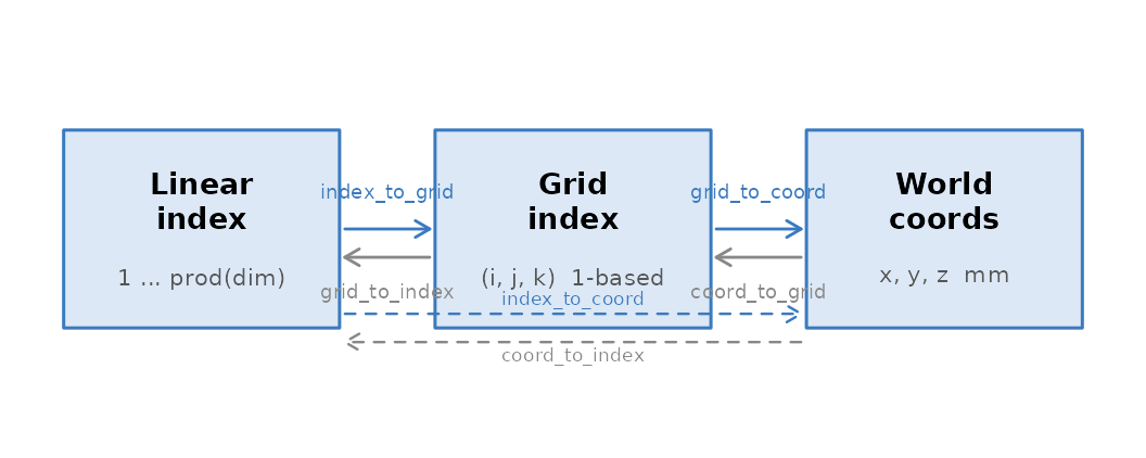
The three addressing schemes and the functions that convert between them.
Coordinate Conversions
All conversion functions accept a NeuroSpace (or any
neuro object, via its attached space) as the first argument.
Grid <-> linear index
# Which linear index does grid position (10, 12, 5) map to?
grid_to_index(sp, matrix(c(10, 12, 5), nrow = 1))
#> [1] 17098

# And back to grid
index_to_grid(sp, 8394L)
#>      [,1] [,2] [,3]
#> [1,]   10    4    3
Grid -> world coordinates
grid_to_coord subtracts 1 from the 1-based grid before
applying the affine, so grid (1, 1, 1) maps exactly to the
origin:
grid_to_coord(sp, matrix(c(1, 1, 1), nrow = 1))   # should equal origin(sp)
#>      [,1] [,2] [,3]
#> [1,]  -90 -126  -72
grid_to_coord(sp, matrix(c(10, 12, 5), nrow = 1))
#>      [,1] [,2] [,3]
#> [1,]  -72 -104  -64
Multiple points are passed as a matrix with one row per point:
pts <- matrix(c(
   1,  1,  1,
  32, 32, 20,
  64, 64, 40
), ncol = 3, byrow = TRUE)

grid_to_coord(sp, pts)
#>      [,1] [,2] [,3]
#> [1,]  -90 -126  -72
#> [2,]  -28  -64  -34
#> [3,]   36    0    6
World -> grid coordinates
coord_to_grid(sp, c(0, 0, 0))          # near isocenter
#> [1] 46 64 37
coord_to_grid(sp, matrix(c(0, 0, 0,
                           10, -20, 8), ncol = 3, byrow = TRUE))
#>      [,1] [,2] [,3]
#> [1,]   46   64   37
#> [2,]   51   54   41
Convenience: linear index <-> world
# Linear index 1 should land at the origin (pass integer)
index_to_coord(sp, 1L)
#>      [,1] [,2] [,3]
#> [1,]  -89 -125  -71

# World coord back to linear index
coord_to_index(sp, matrix(c(-90, -126, -72), nrow = 1))
#> [1] -2079
A concrete round-trip
idx   <- 12345L
grid  <- index_to_grid(sp, idx)
world <- grid_to_coord(sp, grid)
back  <- coord_to_index(sp, world)

cat("index:", idx, "-> grid:", grid, "-> world:", round(world, 2),
    "-> index:", back, "\n")
#> index: 12345 -> grid: 57 1 4 -> world: 22 -126 -66 -> index: 10264
Orientation Codes
Neuroimaging images can be stored in many orientations. The orientation code (also called axis codes or RAS codes) tells you which anatomical direction each image axis points:
| Letter | Anatomical direction |
|---|---|
| R | increasing -> Right |
| L | increasing -> Left |
| A | increasing -> Anterior |
| P | increasing -> Posterior |
| S | increasing -> Superior |
| I | increasing -> Inferior |
A code of "RAS" means: axis 1 runs left-to-right, axis 2
runs posterior-to-anterior, axis 3 runs inferior-to-superior. This is
the standard NIfTI/MNI convention. "LPI" (sometimes called
“neurological”) reverses all three.
affine_to_axcodes() reads the orientation directly from
the affine matrix:
affine_to_axcodes(trans(sp))
#> [1] "R" "A" "S"
The default axis-aligned NeuroSpace built above uses the
nearest-anatomy convention inferred from the affine. You can also
inspect the axes slot directly:
axes(sp)
#> <AxisSet3D>
#>   Axis 1        : Left-to-Right
#>   Axis 2        : Posterior-to-Anterior
#>   Axis 3        : Inferior-to-Superior
Reorienting a space
reorient() flips and permutes the affine to match a
target orientation string:
sp_ras <- reorient(sp, c("R", "A", "S"))
affine_to_axcodes(trans(sp_ras))
#> [1] "L" "P" "I"
Creating NeuroSpaces
From dim + spacing + origin (axis-aligned)
The simplest case: an isotropic or anisotropic grid with no rotation.
# 2 mm isotropic, MNI-ish origin
sp_mni <- NeuroSpace(
  dim     = c(91L, 109L, 91L),
  spacing = c(2, 2, 2),
  origin  = c(-90, -126, -72)
)
sp_mni
#> <NeuroSpace> [3D]
#> ── Geometry ────────────────────────────────────────────────────────────────────
#>   Dimensions    : 91 x 109 x 91
#>   Spacing       : 2 x 2 x 2 mm
#>   Origin        : -90, -126, -72
#>   Orientation   : RAS
#>   Voxels        : 902,629
From an explicit affine
When you have a NIfTI sform/qform matrix, pass it directly:
# Oblique affine: slight off-diagonal terms (scanner tilt)
aff_obl <- matrix(c(
   2.0,  0.2,  0.0,  -90,
   0.0,  2.0,  0.1, -126,
   0.0,  0.0,  2.0,  -72,
   0.0,  0.0,  0.0,    1
), nrow = 4, byrow = TRUE)

sp_obl <- NeuroSpace(dim = c(91L, 109L, 91L), trans = aff_obl)

# spacing() returns column norms — the true physical voxel sizes
spacing(sp_obl)
#> [1] 2.00000 2.00998 2.00250

# diagonal is not exactly 2 mm when the image is tilted
diag(aff_obl[1:3, 1:3])
#> [1] 2 2 2
When does spacing() differ from the affine diagonal?
spacing() always returns the column norms of the 3 × 3
linear block — the physical length of each voxel edge. For a pure
diagonal affine these equal the diagonal entries. For a rotated or
oblique affine they differ. Always use spacing() for
physical voxel sizes; never rely on the diagonal directly.
You can also compute voxel sizes from any affine matrix with
voxel_sizes():
voxel_sizes(aff_obl)
#> [1] 2.000000 2.009975 2.002498
Dimension Manipulation
Adding a time dimension: add_dim
add_dim() extends a 3D NeuroSpace to 4D by
appending a new dimension. The spatial affine is preserved
unchanged:
sp_3d <- NeuroSpace(c(64L, 64L, 40L), spacing = c(2, 2, 2),
                    origin = c(-90, -126, -72))
sp_4d <- add_dim(sp_3d, 200)   # 200 time points
dim(sp_4d)
#> [1]  64  64  40 200
trans(sp_4d)                   # 4x4 spatial affine unchanged
#>      [,1] [,2] [,3] [,4]
#> [1,]    2    0    0  -90
#> [2,]    0    2    0 -126
#> [3,]    0    0    2  -72
#> [4,]    0    0    0    1
Dropping the time dimension: drop_dim
drop_dim() removes the last (or a named) dimension:
sp_back <- drop_dim(sp_4d)
dim(sp_back)
#> [1] 64 64 40
all.equal(trans(sp_back), trans(sp_3d))   # affine preserved
#> [1] TRUE
This round-trip is used internally whenever a 4D volume is sliced to a single time point.
Resampling and Reorientation
resample — change voxel size, keep geometry
resample() resamples a NeuroVol into a
target space (or another volume’s space). To demonstrate, build a small
volume and resample it to a coarser grid:
deoblique — remove scanner tilt
Many scanners acquire data with a slight tilt relative to the MNI
axes. The resulting affine has non-zero off-diagonal elements (an
oblique affine). deoblique() builds an
axis-aligned output space that encloses the original field of view,
using the minimum input voxel size by default (AFNI-style):
sp_deob <- deoblique(sp_obl)
affine_to_axcodes(trans(sp_deob))   # now axis-aligned
#> [1] "R" "A" "S"
obliquity(trans(sp_deob))           # near zero
#> [1] 0 0 0
When passed a NeuroVol, deoblique() also
resamples the image data into the new space.
Common Gotchas
1. Oblique affines and spacing() If
diag(trans(sp)[1:3, 1:3]) does not match
spacing(sp), the affine is oblique. Use
obliquity(trans(sp)) to quantify the tilt angle (in
radians) per axis.
obliquity(aff_obl)        # non-zero: image is slightly tilted
#> [1] 0.00000000 0.09966865 0.04995840
obliquity(trans(sp_mni))  # near zero: axis-aligned
#> [1] 0 0 0
2. 1-based grid indices R uses 1-based indexing.
grid_to_coord() handles this by subtracting 1 before
applying the affine, so voxel (1, 1, 1) lands at
origin(sp). If you ever use raw affine arithmetic, remember
to subtract 1 from your 1-based grid coordinates first.
3. NIfTI sform vs qform NIfTI files store two
possible affines (sform and qform). read_vol() and
read_vec() follow the NIfTI priority rules: sform_code >
0 -> use sform; otherwise use qform. The resulting
trans(space(img)) reflects whichever was chosen. You can
inspect the header with read_header() if you need to see
both.
4. Float32 precision NIfTI stores affine
coefficients as 32-bit floats. neuroim2 rounds the affine to 7
significant figures on construction (signif(trans, 7)) to
match this precision. Round-trip coordinates through
index_to_coord / coord_to_index may therefore
show sub-voxel floating-point noise at the ~0.001 mm level.
Quick Reference
| Function | Input -> Output | Typical use |
|---|---|---|
grid_to_index(sp, mat) |
grid -> linear index | looking up voxel data |
index_to_grid(sp, idx) |
linear index -> grid | converting R array subscripts |
grid_to_coord(sp, mat) |
grid -> mm | overlay on anatomy |
coord_to_grid(sp, mat) |
mm -> grid | atlas lookup |
index_to_coord(sp, idx) |
linear index -> mm | shortcut past grid |
coord_to_index(sp, mat) |
mm -> linear index | mask extraction |
affine_to_axcodes(aff) |
affine -> "RAS" etc. |
orientation check |
voxel_sizes(aff) |
affine -> mm vector | physical voxel size |
obliquity(aff) |
affine -> radians | tilt check |
add_dim(sp, n) |
3D space -> 4D space | attach time axis |
drop_dim(sp) |
4D space -> 3D space | strip time axis |
resample(sp, spacing) |
space -> resampled space | change resolution |
reorient(sp, codes) |
space -> reoriented space | standardise orientation |
deoblique(sp) |
oblique space -> aligned space | remove scanner tilt |
Where to go next
-
vignette("ImageVolumes")— creating and manipulatingNeuroVolobjects -
vignette("NeuroVector")— working with 4D time-series (NeuroVec) -
vignette("Resampling")— image resampling in depth -
vignette("regionOfInterest")— ROI construction and coordinate-based queries -
?NeuroSpace,?affine_to_axcodes,?deoblique— function reference pages