Advanced 3D Volume Patterns

This article is now the detailed follow-on to vignette("VolumesAndVectors"). Read that vignette first if you want the shortest introduction to read_vol(), read_vec(), and the basic NeuroVol / NeuroVec mental model.

Use this article when you specifically want deeper 3D-volume details: masks, coordinate conversion, manual construction, and slice-level inspection.

Read one volume to establish context

file_name <- system.file("extdata", "global_mask2.nii.gz", package = "neuroim2")
vol <- read_vol(file_name)

This article assumes you already know the basic NeuroVol story from vignette("VolumesAndVectors"). The remaining sections focus on patterns that are specific to 3D work.

class(vol)
#> [1] "DenseNeuroVol"
#> attr(,"package")
#> [1] "neuroim2"
is.array(vol)
#> [1] TRUE
dim(vol)
#> [1] 64 64 25
vol[1, 1, 1]
#> [1] 0
vol[64, 64, 24]
#> [1] 0

Coordinate conversion and spatial metadata

sp <- space(vol)
sp
#> <NeuroSpace> [3D] 
#> ── Geometry ──────────────────────────────────────────────────────────────────── 
#>   Dimensions    : 64 x 64 x 25
#>   Spacing       : 3.5 x 3.5 x 3.7 mm
#>   Origin        : 112, -108.5, -46.25
#>   Orientation   : LAS
#>   Voxels        : 102,400
dim(vol)
#> [1] 64 64 25
spacing(vol)
#> [1] 3.5 3.5 3.7
origin(vol)
#> [1]  112.00 -108.50  -46.25

You can convert between indices, voxel grid coordinates, and real-world coordinates:

idx <- 1:5
g <- index_to_grid(vol, idx)
w <- index_to_coord(vol, idx)
idx2 <- coord_to_index(vol, w)
all.equal(idx, idx2)
#> [1] "Mean relative difference: 0.3333333"

A numeric image volume can be converted to a binary image as follows:

vol2 <- as.logical(vol)
class(vol2)
#> [1] "LogicalNeuroVol"
#> attr(,"package")
#> [1] "neuroim2"
print(vol2[1, 1, 1])
#> [1] FALSE

Masks and LogicalNeuroVol

Create a mask from a threshold or an explicit set of indices. Masks are LogicalNeuroVol and align with the 3D space.

mask1 <- as.mask(vol > 0.5)
mask1
#> <DenseNeuroVol> [406.6 Kb] 
#> ── Spatial ───────────────────────────────────────────────────────────────────── 
#>   Dimensions    : 64 x 64 x 25
#>   Spacing       : 3.5 x 3.5 x 3.7 mm
#>   Origin        : 112, -108.5, -46.25
#>   Orientation   : LAS
#> ── Data ──────────────────────────────────────────────────────────────────────── 
#>   Range         : [0.000, 1.000]

idx_hi <- which(vol > 0.8)
mask2 <- as.mask(vol, idx_hi)
sum(mask2) == length(idx_hi)
#> [1] TRUE

mean_in_mask <- mean(vol[mask1@.Data])
mean_in_mask
#> [1] 1

Constructing volumes manually

We can also create a NeuroVol instance from an array or numeric vector. First we construct a standard R array:

    x <- array(0, c(64,64,64))

Now we create a NeuroSpace instance that describes the geometry of the image, including at minimum its dimensions and voxel spacing.

    bspace <- NeuroSpace(dim=c(64,64,64), spacing=c(1,1,1))
    vol <- NeuroVol(x, bspace)
    vol
#> <DenseNeuroVol> [2 Mb] 
#> ── Spatial ───────────────────────────────────────────────────────────────────── 
#>   Dimensions    : 64 x 64 x 64
#>   Spacing       : 1 x 1 x 1 mm
#>   Origin        : 0, 0, 0
#>   Orientation   : RAS
#> ── Data ──────────────────────────────────────────────────────────────────────── 
#>   Range         : [0.000, 0.000]

We do not usually have to create NeuroSpace objects by hand because real image files carry this information in their headers. In practice you usually copy an existing space:

    vol2 <- NeuroVol((vol+1)*25, space(vol))
    max(vol2)
#> [1] 25
    space(vol2)
#> <NeuroSpace> [3D] 
#> ── Geometry ──────────────────────────────────────────────────────────────────── 
#>   Dimensions    : 64 x 64 x 64
#>   Spacing       : 1 x 1 x 1 mm
#>   Origin        : 0, 0, 0
#>   Orientation   : RAS
#>   Voxels        : 262,144

Slicing and quick visualization

The easiest way to view a volume is with plot(), which shows a 3 x 3 montage of evenly-spaced axial slices:

plot(vol)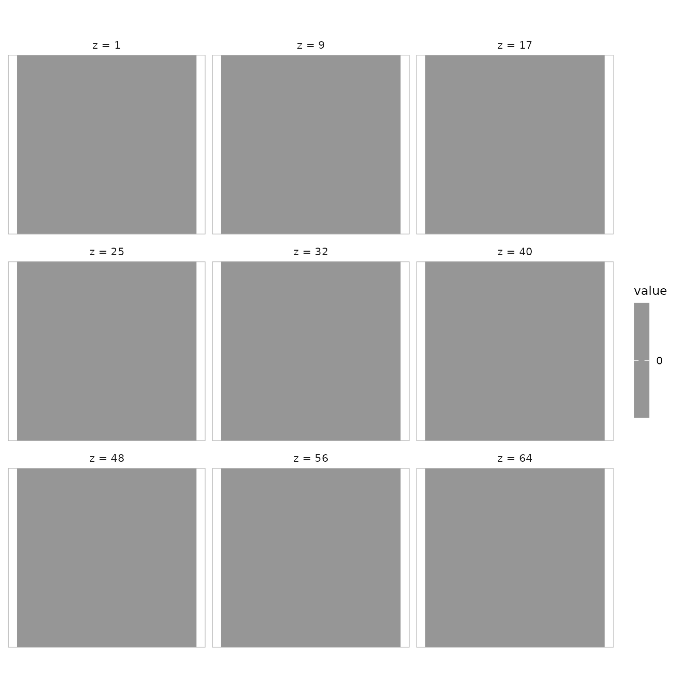

Default plot() montage

You can also extract a single 2D slice for display using standard array indexing:

    z <- ceiling(dim(vol)[3] / 2)
    image(vol[,,z], main = paste("Slice z=", z))

Mid-slice of example volume

Reorienting and resampling

You can change an image’s orientation and voxel spacing. Use reorient() to remap axes (e.g., to RAS) and resample_to() to match a target space.

    # Reorient the space (LPI -> RAS) and compare coordinate mappings
    sp_lpi <- space(vol)
    sp_ras <- reorient(sp_lpi, c("R","A","S"))
    g     <- t(matrix(c(10, 10, 10)))
    world_lpi <- grid_to_coord(sp_lpi, g)
    world_ras <- grid_to_coord(sp_ras, g)
    # world_lpi and world_ras differ due to axis remapping

Resample to a new spacing or match a target NeuroSpace:

    # Create a target space with 2x finer resolution
    sp  <- space(vol)
    sp2 <- NeuroSpace(sp@dim * c(2,2,2), sp@spacing/2, origin=sp@origin, trans=trans(vol))

    # Resample (trilinear)
    vol_resamp <- resample_to(vol, sp2, method = "linear")
    dim(vol_resamp)

Downsampling

Reduce spatial resolution to speed up downstream operations.

    # Downsample by target spacing
    vol_ds1 <- downsample(vol, spacing = spacing(vol)[1:3] * 2)
    dim(vol_ds1)
#> [1] 32 32 32

    # Or by factor
    vol_ds2 <- downsample(vol, factor = 0.5)
    dim(vol_ds2)
#> [1] 32 32 32

Writing a NIFTI formatted image volume

When we’re ready to write an image volume to disk, we use write_vol

    write_vol(vol2, "output.nii")
    
    ## adding a '.gz' extension results ina gzipped file.
    write_vol(vol2, "output.nii.gz")

You can also write to a temporary file during workflows:

    tmp <- tempfile(fileext = ".nii.gz")
    write_vol(vol2, tmp)
    file.exists(tmp)
#> [1] TRUE
    unlink(tmp)

For reorientation, resampling, and downsampling, use vignette("Resampling"), which now owns that topic directly.

2026-04-16