Multiple Factor Analysis

Why MFA?

Multiple Factor Analysis (MFA) solves a common problem: you have measured the same observations using different instruments, different feature sets, or at different time points — and you want a single, integrated view. Standard PCA on the concatenated data fails here because blocks with more variables or higher variance dominate the solution. MFA corrects this by normalizing each block before integration, so every data source contributes fairly.

MFA belongs to the “French school” of multivariate analysis, developed by Escofier and Pagès in the 1980s. It remains one of the most principled approaches for multi-table data integration.

Quick start

library(muscal)
library(multivarious)
library(ggplot2)

Generate four blocks of data that share three latent components. Each block has a different number of variables — exactly the situation where plain PCA on the concatenated data would be misleading.

sim <- synthetic_multiblock(
  S = 4, n = 60,
  p = c(20, 30, 15, 25),
  r = 3, sigma = 0.3, seed = 42
)
sapply(sim$data_list, dim)
#>      [,1] [,2] [,3] [,4]
#> [1,]   60   60   60   60
#> [2,]   20   30   15   25

Fit MFA and extract the compromise scores:

fit <- mfa(sim$data_list, ncomp = 3)
S <- scores(fit)
dim(S)
#> [1] 60  3

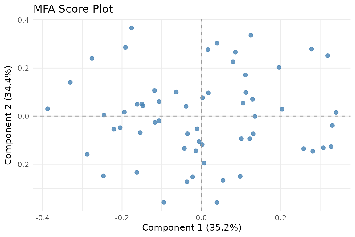
Observations in the MFA compromise space. The first two components capture the dominant shared structure across all four blocks.

The score plot shows 60 observations positioned according to their combined profile across all four blocks. Components 1 and 2 explain the largest portion of shared variance.

The core idea

MFA proceeds in two stages:

1. Normalize each block so that no single block dominates. The default approach divides each block by its first singular value — this makes the maximum inertia of each block equal to 1.

2. Apply PCA to the concatenated, normalized blocks to extract global components that summarize the shared structure across all data sources.

The result is a compromise factor space where observations are positioned according to their combined profile across all blocks.

Working with the results

The MFA result is a multiblock_biprojector from the multivarious package. You can access global scores, block-specific loadings, and normalization weights:

head(S, 4)
#>              PC1        PC2        PC3
#> Obs1  0.11216956 0.09830377 -0.4334275
#> Obs2  0.01771288 0.09650491 -0.1327023
#> Obs3 -0.14997782 0.05007061  0.3016705
#> Obs4  0.31836131 0.25117706 -0.1006403

# Normalization weights — blocks with more variables get smaller weights
fit$alpha
#>         B1         B2         B3         B4 
#> 0.07002450 0.06521398 0.09453764 0.06909297

Notice how blocks with 30 and 25 variables (blocks 2 and 4) receive smaller weights than the block with 15 variables (block 3). This is MFA’s key balancing act.

Block-specific loadings are slices of the concatenated loading matrix, indexed by block_indices:

str(fit$block_indices)
#> List of 4
#>  $ : int [1:20] 1 2 3 4 5 6 7 8 9 10 ...
#>  $ : int [1:30] 21 22 23 24 25 26 27 28 29 30 ...
#>  $ : int [1:15] 51 52 53 54 55 56 57 58 59 60 ...
#>  $ : int [1:25] 66 67 68 69 70 71 72 73 74 75 ...

Visualization

muscal provides several plotting functions that work with both base R and ggplot2. When ggplot2 is loaded, most functions return ggplot objects.

Score plot

The primary visualization shows observations in the compromise space. You can color points by an external variable to look for group structure:

groups <- rep(c("A", "B", "C"), length.out = 60)
autoplot(fit, color = groups)

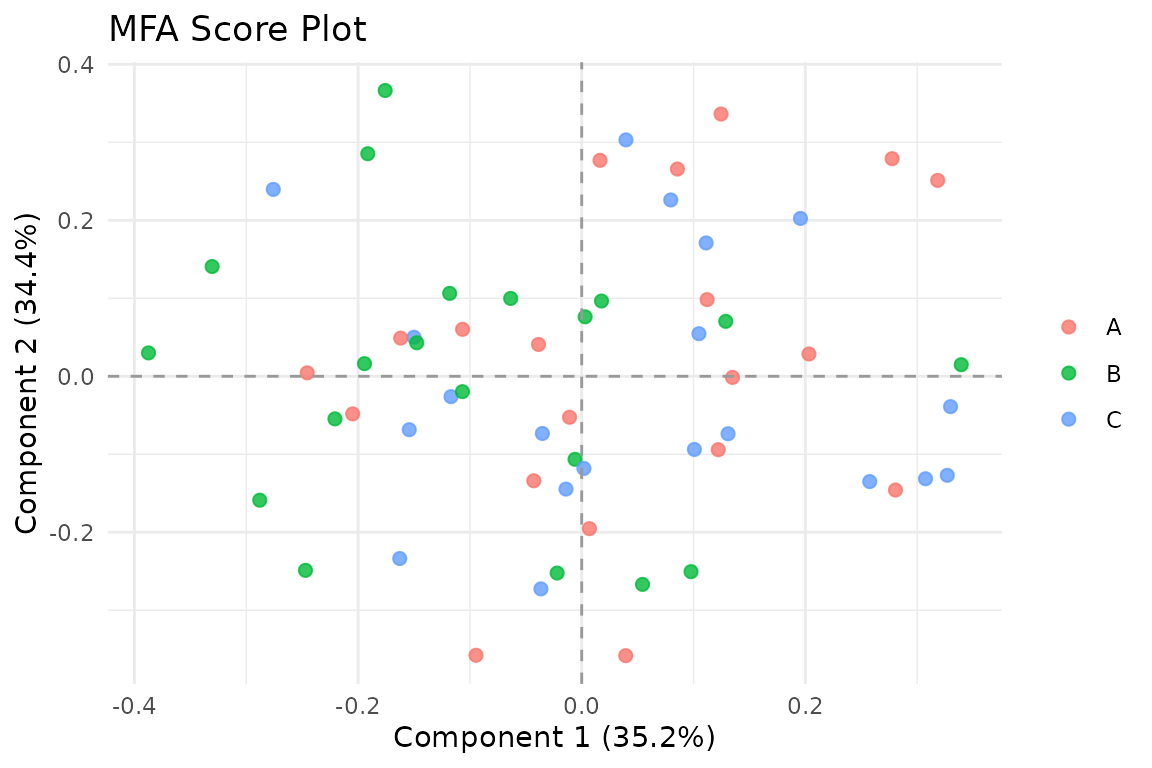
Score plot colored by a grouping variable.

Variance explained

Assess how the retained components distribute variance:

plot_variance(fit, type = "bar")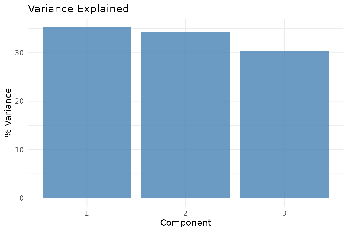

Proportion of variance captured by each retained component in the three-component MFA solution.

Block weights

Understand the normalization effect:

plot_block_weights(fit)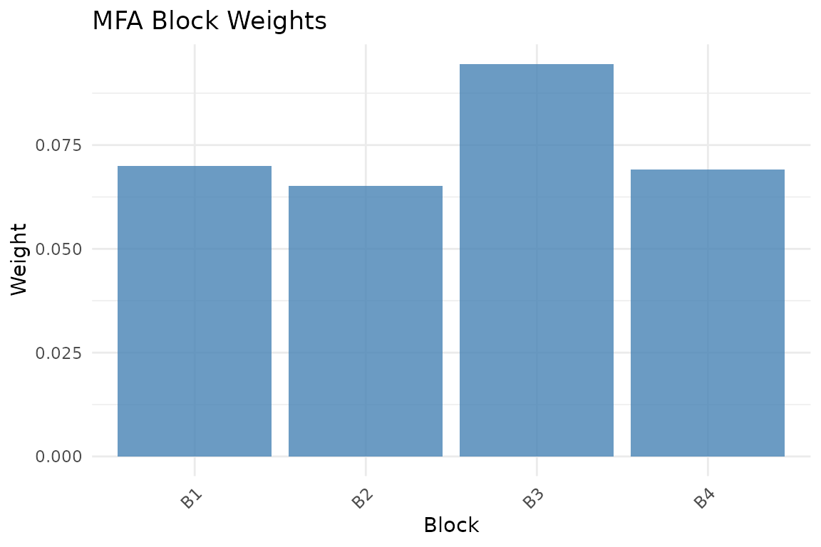

MFA normalization weights. Blocks with smaller first singular values receive larger weights, equalizing their contribution.

Partial factor scores

Each block has its own “view” of the observations. Partial factor scores show where each block would place the observations, connected to the consensus position. In a dense plot like this one, focus on the overall spread of the segments rather than trying to read every observation individually:

plot_partial_scores(fit, connect = TRUE, show_consensus = TRUE)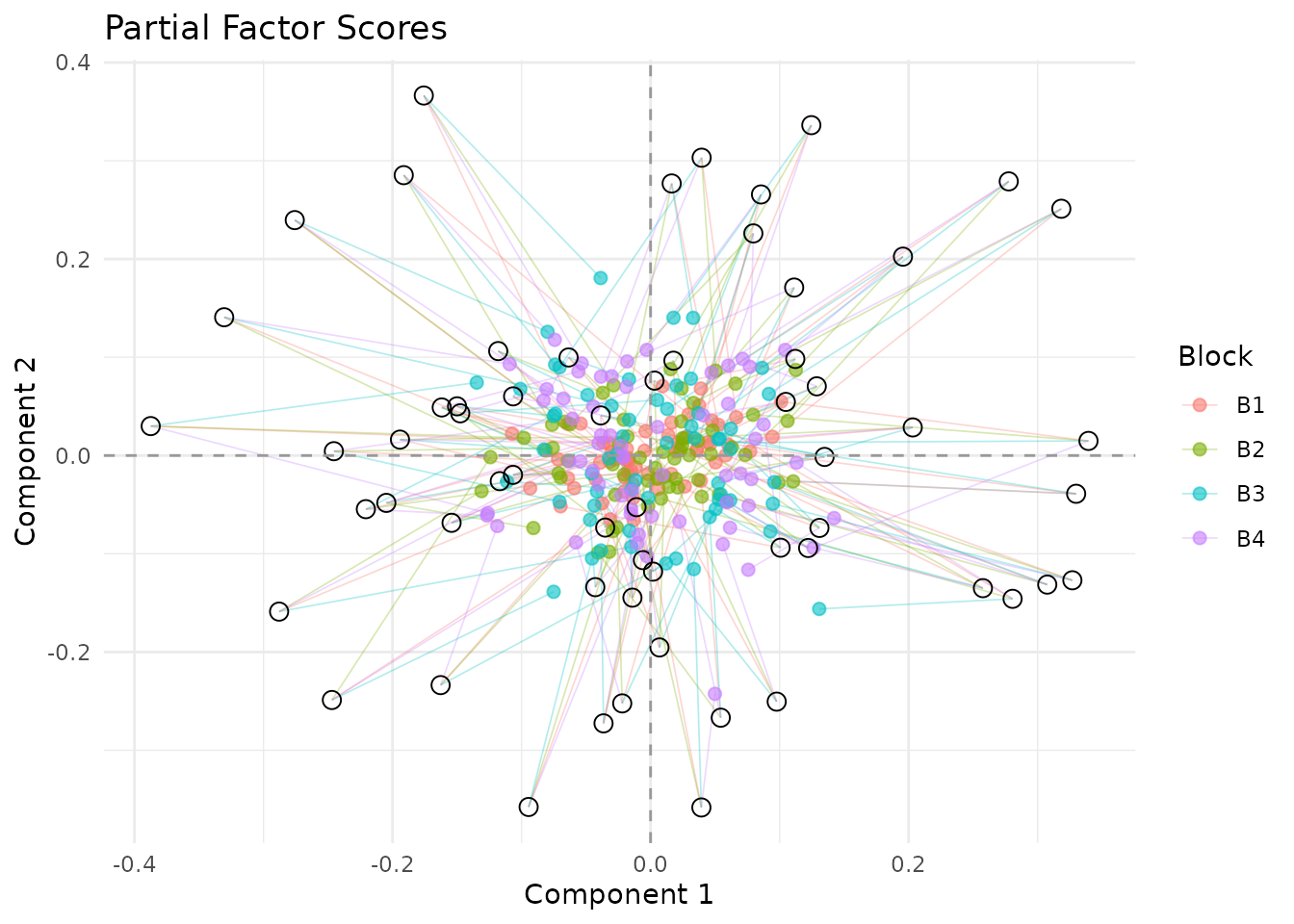

Partial factor scores. Lines connect each block’s view to the consensus; tighter clouds and shorter segments indicate stronger agreement across blocks.

Observations with long segments are cases where one or more blocks disagree more strongly with the compromise position.

Block similarity

The RV coefficient matrix shows how similar the blocks are to each other:

plot_block_similarity(fit, method = "RV")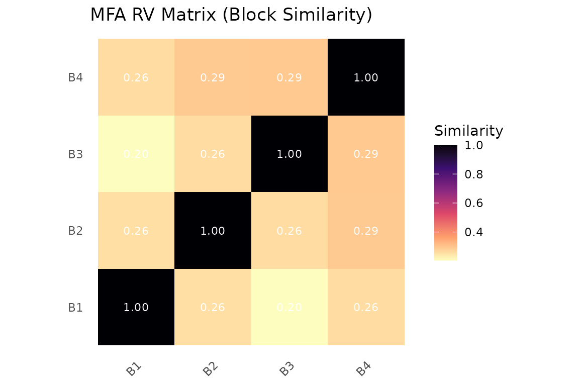

RV coefficient matrix. Values near 1 indicate blocks that carry similar information.

Variable loadings

Visualize which variables drive each component:

plot_loadings(fit, type = "bar", component = 1, top_n = 15)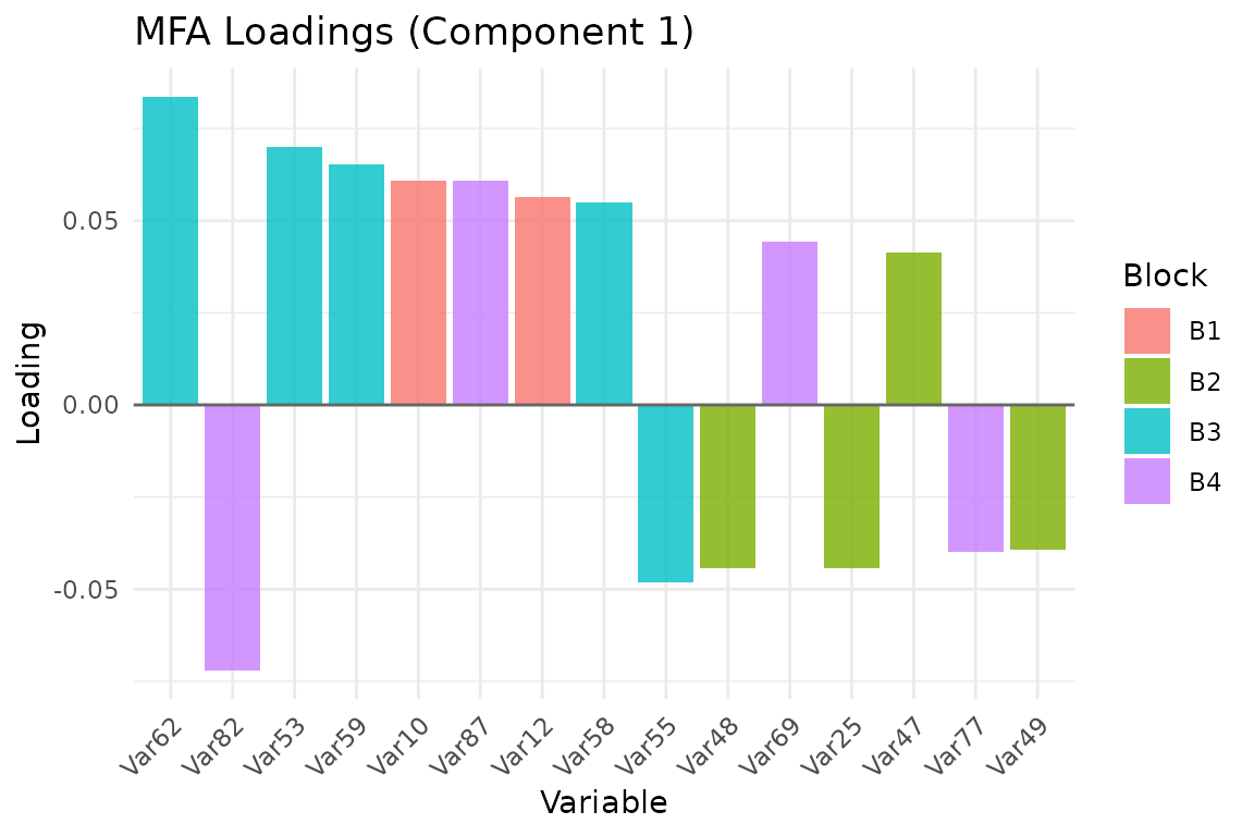

Top 15 variable loadings on component 1, colored by block membership.

Normalization schemes

MFA supports several block-weighting schemes via the normalization argument:

• "MFA" (default): Weight by inverse squared first singular value. This is the classical MFA normalization.

• "RV": Weight blocks by their contribution to the RV coefficient matrix. Blocks more similar to the overall structure receive higher weight.

• "Frob": Weight by Frobenius norm.

• "None": No normalization — equivalent to ordinary PCA on concatenated data.

• "custom": Supply your own weight matrices via A (column weights) and M (row weights).

# RV-based normalization
fit_rv <- mfa(sim$data_list, ncomp = 3, normalization = "RV")

# Custom weights: inverse-column-count weighting
ncols <- sapply(sim$data_list, ncol)
custom_weights <- rep(1 / ncols, ncols)
fit_custom <- mfa(sim$data_list, ncomp = 3,
                  normalization = "custom", A = custom_weights)

Inference and validation

MFA is exploratory, but the package also supports resampling-based diagnostics and held-out reconstruction checks. These are useful when you want to know whether the leading components are stable and whether the fitted compromise generalizes to unseen rows.

boot <- infer_muscal(
  fit,
  method = "bootstrap",
  statistic = "sdev",
  nrep = 8,
  seed = 101
)

boot$summary
#> # A tibble: 3 × 7
#>   component label observed  mean     sd lower upper
#>       <int> <chr>    <dbl> <dbl>  <dbl> <dbl> <dbl>
#> 1         1 comp1     1.38  1.59 0.0758  1.52  1.74
#> 2         2 comp2     1.37  1.42 0.0665  1.34  1.52
#> 3         3 comp3     1.28  1.35 0.0680  1.24  1.45

perm <- infer_muscal(
  fit,
  method = "permutation",
  statistic = "sdev",
  nrep = 19,
  seed = 202
)

perm$component_results
#> # A tibble: 3 × 6
#>   component label observed p_value lower_ci upper_ci
#>       <int> <chr>    <dbl>   <dbl>    <dbl>    <dbl>
#> 1         1 comp1     1.38    0.6      1.34     1.44
#> 2         2 comp2     1.37    0.1      1.30     1.36
#> 3         3 comp3     1.28    0.95     1.28     1.34

stopifnot(all(is.finite(boot$summary$mean)))
stopifnot(all(boot$summary$upper >= boot$summary$lower))
stopifnot(all(perm$component_results$p_value >= 0))
stopifnot(all(perm$component_results$p_value <= 1))

For held-out evaluation, use cv_muscal() with row folds and reconstruction metrics:

X_concat <- do.call(cbind, sim$data_list)
md <- multidesign::multidesign(X_concat, data.frame(batch = rep(c("A", "B"), each = 30)))
folds <- multidesign::cv_rows(md, rows = list(1:6, 31:36), preserve_row_ids = TRUE)

res_cv <- cv_muscal(
  folds = folds,
  fit_fn = function(analysis) {
    Xa <- multidesign::xdata(analysis)
    mfa(
      list(
        X1 = Xa[, 1:20, drop = FALSE],
        X2 = Xa[, 21:50, drop = FALSE],
        X3 = Xa[, 51:65, drop = FALSE],
        X4 = Xa[, 66:90, drop = FALSE]
      ),
      ncomp = 3
    )
  },
  estimate_fn = function(model, assessment) {
    predict(model, multidesign::xdata(assessment), type = "reconstruction")
  },
  truth_fn = function(assessment) multidesign::xdata(assessment),
  metrics = c("mse", "rmse", "r2")
)

res_cv$scores
#> # A tibble: 2 × 4
#>      mse  rmse      r2 .fold
#>    <dbl> <dbl>   <dbl> <int>
#> 1 0.101  0.318 -0.0364     1
#> 2 0.0911 0.302 -0.0233     2

stopifnot(all(is.finite(res_cv$scores$mse)))
stopifnot(all(res_cv$scores$rmse >= 0))

For a fuller walkthrough of infer_muscal(), cv_muscal(), and the available metric families, see vignette("model_evaluation").

When to use MFA

MFA is appropriate when:

• You have multiple measurement modalities on the same subjects (e.g., gene expression + metabolomics + clinical variables).
• You want to identify patterns that are consistent across data sources.
• You need block contributions to be balanced regardless of the number of variables per block.

MFA is not appropriate when:

• Blocks have different observations (use anchored_mfa() instead).
• You want blocks with more variables to naturally dominate (use standard PCA).
• Your goal is prediction rather than exploratory structure discovery.

Next steps

• vignette("linked_mfa") — Continue to Anchored MFA when your blocks no longer share the same observations
• vignette("model_evaluation") — Bootstrap, permutation, and held-out evaluation workflows across supported methods
• vignette("ipca") — Compare MFA with adaptive block reweighting in Integrative PCA
• vignette("mcca") — Switch to a correlation-driven shared score space when cross-block agreement matters more than balanced variance
• vignette("penalized_mfa") — Add structure-aware penalties to the MFA framework

References

Escofier, B., & Pagès, J. (1994). Multiple factor analysis (AFMULT package). Computational Statistics & Data Analysis, 18(1), 121-140.

Abdi, H., Williams, L. J., & Valentin, D. (2013). Multiple factor analysis: Principal component analysis for multitable and multiblock data sets. Wiley Interdisciplinary Reviews: Computational Statistics, 5(2), 149-179.