Integrative PCA (iPCA) • muscal

Why iPCA?

When you run PCA on concatenated multi-block data, blocks with more variables or higher variance dominate the result. MFA addresses this by normalizing each block’s first singular value to 1. But this is a single global correction — it doesn’t adapt to the actual signal content of each block.

Integrative PCA (iPCA) takes a different approach. It applies per-block multiplicative penalties that continuously reweight each block’s contribution based on how well it aligns with the emerging shared structure. The penalty strength lambda controls how aggressively blocks are equalized: small lambda approaches standard PCA, large lambda gives each block equal influence regardless of size.

iPCA was introduced by Tang and Allen (2021) and implemented here using an efficient Flip-Flop algorithm.

Quick start

library(muscal)
library(multivarious)
library(ggplot2)

sim <- synthetic_multiblock(
  S = 4, n = 60,
  p = c(20, 30, 15, 25),
  r = 3, sigma = 0.3, seed = 42
)
sapply(sim$data_list, dim)
#>      [,1] [,2] [,3] [,4]
#> [1,]   60   60   60   60
#> [2,]   20   30   15   25

Fit iPCA with a moderate penalty:

fit <- ipca(sim$data_list, ncomp = 3, lambda = 1)
S <- scores(fit)
dim(S)
#> [1] 60  3

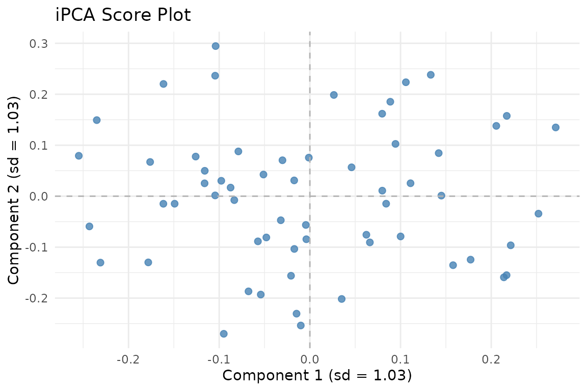
iPCA scores. The multiplicative penalty balances block contributions while preserving shared structure.

How iPCA works

iPCA solves a penalized eigenvalue problem. For $K$ blocks $\mathbf{X}_1, \ldots, \mathbf{X}_K$ , it finds shared eigenvectors $u$ by maximizing:

$\sum_{k=1}^K f_\lambda\!\left(\frac{u^\top \mathbf{X}_k^\top \mathbf{X}_k\, u} {\mathrm{tr}(\mathbf{X}_k^\top \mathbf{X}_k)}\right)$

where $f_\lambda$ is a concave penalty function (the multiplicative Frobenius penalty). This upweights blocks that align well with the current direction and downweights those that don’t — a soft, adaptive form of integration.

The lambda parameter

lambda controls the integration strength:

lambda near 0: Standard PCA on concatenated data (no reweighting). Blocks with more variables dominate.
lambda = 1: Moderate integration. Blocks are softly equalized.
Large lambda (10+): Strong equalization. Every block contributes roughly equally, regardless of size.

fit_low  <- ipca(sim$data_list, ncomp = 3, lambda = 0.01)
fit_high <- ipca(sim$data_list, ncomp = 3, lambda = 10)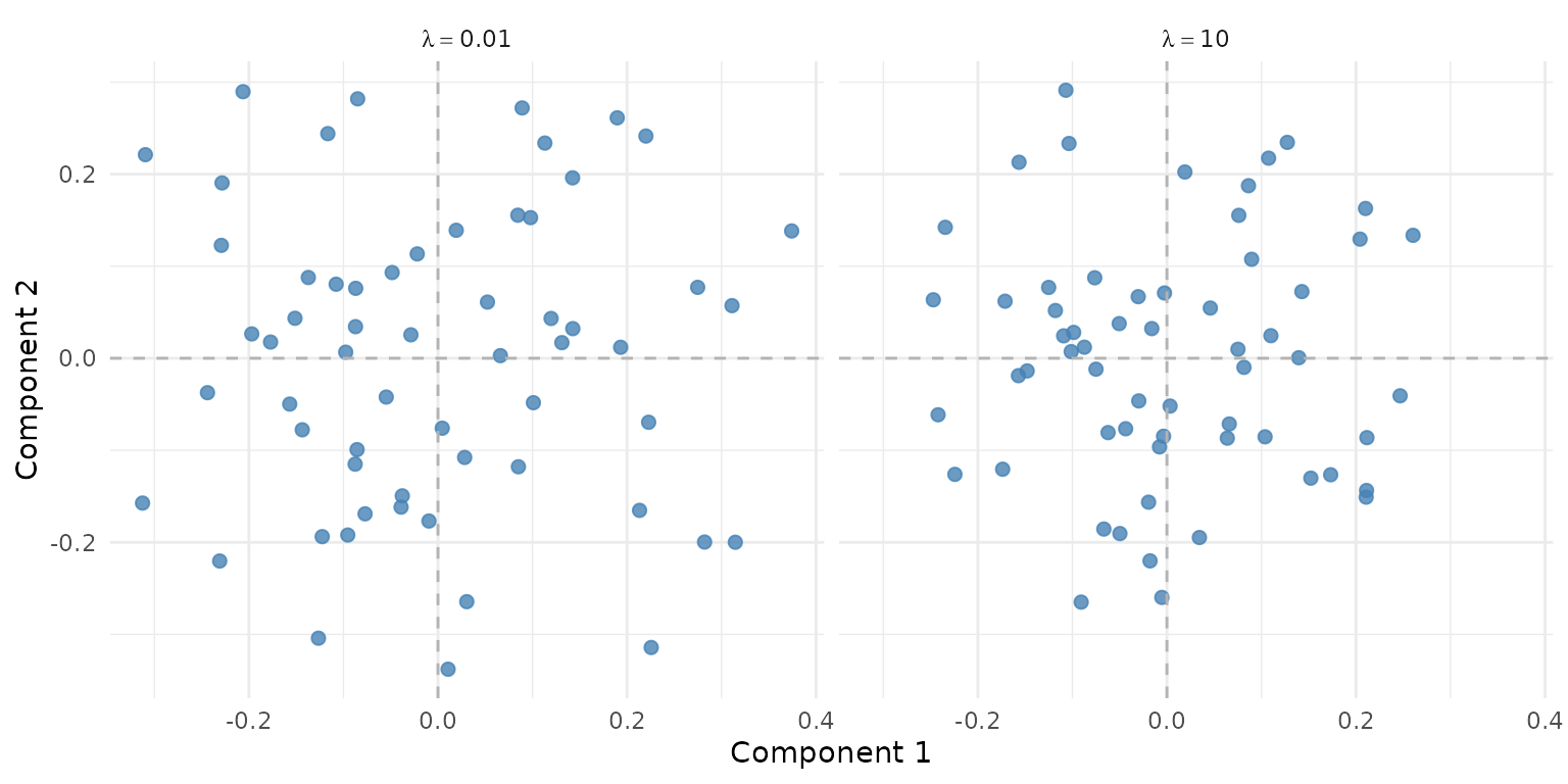

Effect of lambda on the score space. Low lambda (left) lets larger blocks dominate; high lambda (right) equalizes contributions.

Tuning lambda with held-out data

ipca_tune_alpha() selects the optimal penalty by holding out a fraction of the data and measuring reconstruction error:

tune <- ipca_tune_alpha(
  sim$data_list, ncomp = 3,
  alpha_grid = c(0.01, 0.1, 1, 10),
  holdout_frac = 0.1
)
tune$best_alpha
#> [1] 10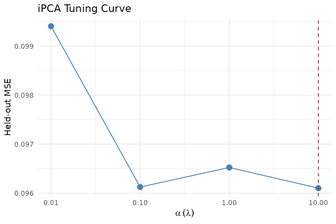

Held-out MSE across alpha (lambda) values. Lower is better.

The tuning result includes a refit on the full data at the best alpha:

fit_tuned <- tune$fit
dim(scores(fit_tuned))
#> [1] 60  3

Partial scores

Each block contributes its own view of the observations through per-block loadings:

# Per-block scores
ps <- fit$partial_scores
sapply(ps, dim)
#>      B1 B2 B3 B4
#> [1,] 60 60 60 60
#> [2,]  3  3  3  3

Projection

Project new observations onto the fitted model. You pass a list of blocks with the same structure as the training data:

new_blocks <- lapply(sim$data_list, function(X) X[1:5, , drop = FALSE])
proj <- project(fit, new_blocks)
dim(proj)
#> [1] 5 3

Inference and validation

iPCA now participates in the same generic evaluation surface as MFA. Use infer_muscal() for resampling-based summaries, and cv_muscal() when you want explicit fold-wise reconstruction metrics.

boot <- infer_muscal(
  fit,
  method = "bootstrap",
  statistic = "sdev",
  nrep = 6,
  seed = 303
)

boot$summary
#> # A tibble: 3 × 7
#>   component label observed  mean      sd lower upper
#>       <int> <chr>    <dbl> <dbl>   <dbl> <dbl> <dbl>
#> 1         1 comp1     1.03  1.07 0.0134   1.06  1.09
#> 2         2 comp2     1.03  1.06 0.00881  1.05  1.07
#> 3         3 comp3     1.03  1.05 0.00476  1.04  1.05

perm <- infer_muscal(
  fit,
  method = "permutation",
  statistic = "sdev",
  nrep = 9,
  seed = 404
)

perm$component_results
#> # A tibble: 3 × 6
#>   component label observed p_value lower_ci upper_ci
#>       <int> <chr>    <dbl>   <dbl>    <dbl>    <dbl>
#> 1         1 comp1     1.03     0.8     1.03     1.04
#> 2         2 comp2     1.03     0.7     1.03     1.03
#> 3         3 comp3     1.03     0.8     1.03     1.03

stopifnot(all(is.finite(boot$summary$mean)))
stopifnot(all(boot$summary$upper >= boot$summary$lower))
stopifnot(all(perm$component_results$p_value >= 0))
stopifnot(all(perm$component_results$p_value <= 1))

For a package-level walkthrough of infer_muscal(), cv_muscal(), and the task-aware metric registry, see vignette("model_evaluation").

Computation methods

iPCA supports two internal methods:

"gram" (default for wide data): Works in sample space ( $n \times n$ ). Efficient when blocks have more variables than observations.
"dense": Works in variable space. Better for tall data.

The "auto" setting (default) picks the right method based on data dimensions.

# Force gram mode for high-dimensional blocks
fit_gram <- ipca(sim$data_list, ncomp = 3, lambda = 1, method = "gram")

When to use iPCA

iPCA is appropriate when:

You have multiple data blocks on the same observations
You want adaptive, data-driven integration (vs. MFA’s fixed normalization)
Blocks vary substantially in dimensionality or signal strength
You want a tunable integration strength

iPCA is not appropriate when:

Blocks have different observations (use anchored_mfa())
You need classical MFA block weights for interpretation (use mfa())
Your data are covariance matrices (use covstatis())

Next steps

vignette("mfa") — Classical MFA with fixed normalization
vignette("model_evaluation") — Generic inference and held-out evaluation workflows
vignette("penalized_mfa") — MFA with loading similarity penalties
?ipca_tune_alpha — Detailed tuning options

References

Tang, T. M., & Allen, G. I. (2021). Integrated principal components analysis. Journal of Machine Learning Research, 22(224), 1-71.