Why MCCA?
Use mcca() when you have several blocks measured on the
same observations and you care about the shared score space
rather than raw variance in the concatenated data. The method looks for
components that each block can project onto coherently, so it is a
natural choice when blocks differ in scale or dimensionality but should
still agree on the same latent structure.
If your main question is “what common signal do these blocks line up
on?”, MCCA is a strong next step after vignette("mfa") when
correlation structure matters more than variance balancing.
What does a quick fit look like?
sapply(blocks, dim)
#>      clinical behavior imaging
#> [1,]       80       80      80
#> [2,]       16       20      18
fit <- mcca(blocks, ncomp = 2, ridge = 1e-6)
S <- multivarious::scores(fit)

stopifnot(all(dim(S) == c(n, 2)))
stopifnot(all(is.finite(S)))
cc <- cancor(
  scale(Z, center = TRUE, scale = FALSE),
  scale(S, center = TRUE, scale = FALSE)
)$cor[1:2]

stopifnot(all(is.finite(cc)))
stopifnot(min(cc) > 0.9)

round(cc, 3)
#> [1] 0.999 0.998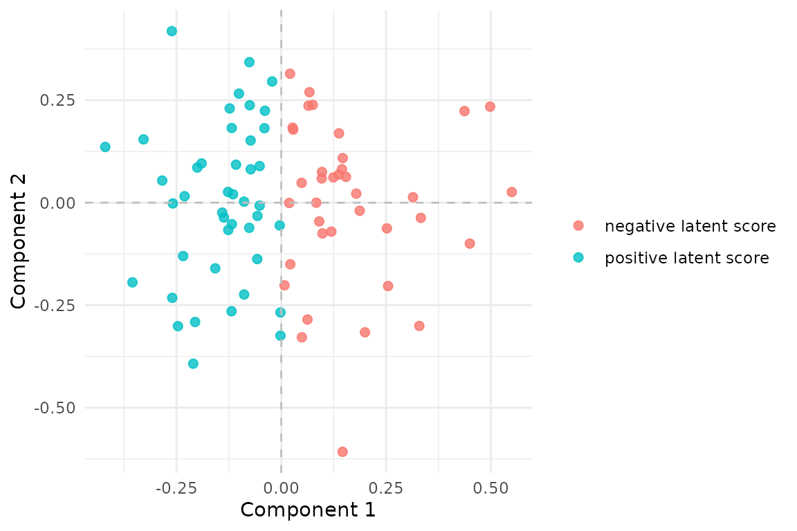
MCCA scores recover the shared low-dimensional structure. The coloring is derived from the first latent factor used to generate the blocks.
The canonical correlations above are the first sanity check. In this simulated example, the fitted scores recover the two shared latent directions very strongly.
What is the method actually doing?
MCCA builds a compromise score space that all blocks can project into. In the MAXVAR formulation used here, each block contributes a ridge-stabilized projection operator, and the shared components are the leading eigenvectors of their weighted sum.
That is why mcca() stays stable even when some blocks
are wide (p >> n) or close to rank-deficient after
centering.
What should you inspect after fitting?
sapply(fit$partial_scores, dim)
#>      clinical behavior imaging
#> [1,]       80       80      80
#> [2,]        2        2       2
S_sum <- Reduce(`+`, fit$partial_scores)
max_diff <- max(abs(S_sum - S))

stopifnot(is.finite(max_diff))
stopifnot(max_diff < 1e-6)

max_diff
#> [1] 2.965363e-10
Each block has its own partial score matrix. Their sum reproduces the compromise scores, so large disagreements across partial scores tell you where the blocks are pulling in different directions.
Inference and validation
MCCA now participates in the same generic evaluation surface as MFA and iPCA. For this method, the most natural resampling question is whether the shared score space is more coherent than what you would get after breaking row alignment across blocks.
boot <- infer_muscal(
  fit,
  method = "bootstrap",
  statistic = "sdev",
  nrep = 6,
  seed = 303
)

boot$summary
#> # A tibble: 2 × 7
#>   component label observed  mean       sd lower upper
#>       <int> <chr>    <dbl> <dbl>    <dbl> <dbl> <dbl>
#> 1         1 comp1     1.73  1.73 0.000175  1.73  1.73
#> 2         2 comp2     1.73  1.73 0.000385  1.73  1.73
perm <- infer_muscal(
  fit,
  method = "permutation",
  statistic = "sdev",
  nrep = 9,
  seed = 404
)

perm$component_results
#> # A tibble: 2 × 6
#>   component label observed p_value lower_ci upper_ci
#>       <int> <chr>    <dbl>   <dbl>    <dbl>    <dbl>
#> 1         1 comp1     1.73     0.1     1.51     1.56
#> 2         2 comp2     1.73     0.1     1.49     1.53
stopifnot(all(is.finite(boot$summary$mean)))
stopifnot(all(boot$summary$upper >= boot$summary$lower))
stopifnot(all(perm$component_results$p_value >= 0))
stopifnot(all(perm$component_results$p_value <= 1))
Because mcca() is a same-row model, you can also score
held-out rows with the generic reconstruction workflow shown in
vignette("model_evaluation").
When should you reach for MCCA?
Use mcca() when:
- your blocks share the same rows,
- you want a common score space driven by cross-block agreement,
- some blocks are much wider than others, and
- you need ridge stabilization in high dimensions.
Use mfa() instead when you want a classical
variance-balancing factor model rather than a canonical-correlation
view.
Where next?
-
vignette("mfa")for variance-based multiblock integration -
vignette("model_evaluation")for generic inference and held-out evaluation workflows -
vignette("aligned_mcca")for the same idea when blocks do not share the same rows -
?mccafor tuningridgeandblock_weights