Working with Clustered fMRI Data: H5ClusterExperiment

library(fmristore)
#> 
#> Attaching package: 'fmristore'
#> The following object is masked from 'package:stats':
#> 
#>     offset
library(neuroim2)
#> Loading required package: Matrix
#> 
#> Attaching package: 'neuroim2'
#> The following object is masked from 'package:base':
#> 
#>     scale

Overview

The H5ClusterExperiment class provides an efficient way to store and access multi-run fMRI data that has been organized by spatial clusters (e.g., brain parcels or regions). This approach is particularly useful when:

You have multiple fMRI runs from the same or different subjects
Your data has been parcellated using an atlas or clustering algorithm
You want efficient access to time series from specific brain regions
You need to store both full voxel-level data and summary statistics

Key Concepts

What is Clustered Data?

Instead of storing fMRI data as a regular 4D array (x, y, z, time), clustered storage groups voxels by their cluster membership. This provides:

Faster access to all voxels within a brain region
Efficient storage through better compression of similar signals
Flexible analysis at both voxel and region levels

Types of Cluster Runs

Full Runs (H5ClusterRun): Store complete time series for every voxel
Summary Runs (H5ClusterRunSummary): Store only averaged time series per cluster

Creating an H5ClusterExperiment

Let’s start with a simple example using simulated data.

Step 1: Define the Brain Space

# Create a small brain volume (10x10x5 voxels)
brain_dim <- c(10, 10, 5)
brain_space <- NeuroSpace(brain_dim, spacing = c(2, 2, 2))

# Create a mask (which voxels contain brain tissue)
mask_data <- array(FALSE, brain_dim)
mask_data[3:8, 3:8, 2:4] <- TRUE  # Simple box-shaped "brain"

mask <- LogicalNeuroVol(mask_data, brain_space)
cat("Number of brain voxels:", sum(mask), "\n")
#> Number of brain voxels: 108

Step 2: Define Clusters

# Create 3 clusters within the mask
n_voxels <- sum(mask)
cluster_ids <- rep(1:3, length.out = n_voxels)

# Create the clustered volume
clusters <- ClusteredNeuroVol(mask, cluster_ids)

# Check cluster sizes
table(clusters@clusters)
#> 
#>  1  2  3 
#> 36 36 36

Step 3: Prepare Run Data

Now let’s create data for two fMRI runs - one with full voxel data and one with summary data.

# Run 1: Full voxel-level data
n_timepoints_run1 <- 100

# Create data for each cluster
run1_data <- list()
for (cid in 1:3) {
  voxels_in_cluster <- sum(clusters@clusters == cid)
  # Simulate time series with cluster-specific patterns
  run1_data[[paste0("cluster_", cid)]] <-
    matrix(rnorm(voxels_in_cluster * n_timepoints_run1,
      mean = cid),  # Different mean for each cluster
    nrow = voxels_in_cluster,
    ncol = n_timepoints_run1)
}

# Run 2: Summary data (averaged time series per cluster)
n_timepoints_run2 <- 150
run2_data <- matrix(rnorm(n_timepoints_run2 * 3),
  nrow = n_timepoints_run2,
  ncol = 3)

Step 4: Create Metadata

# Metadata for each run
run1_metadata <- list(
  subject_id = "sub-01",
  task = "rest",
  TR = 2.0
)

run2_metadata <- list(
  subject_id = "sub-01",
  task = "motor",
  TR = 2.0
)

# Cluster metadata
cluster_metadata <- data.frame(
  cluster_id = 1:3,
  name = c("Visual", "Motor", "Default"),
  color = c("red", "green", "blue")
)

Step 5: Write to HDF5

# Prepare the runs data structure
runs_data <- list(
  list(
    scan_name = "rest_run",
    type = "full",
    data = run1_data,
    metadata = run1_metadata
  ),
  list(
    scan_name = "motor_run",
    type = "summary",
    data = run2_data,
    metadata = run2_metadata
  )
)

# Write to HDF5
h5_file <- tempfile(fileext = ".h5")
write_clustered_experiment_h5(
  filepath = h5_file,
  mask = mask,
  clusters = clusters,
  runs_data = runs_data,
  cluster_metadata = cluster_metadata,
  overwrite = TRUE,
  verbose = FALSE
)

Reading and Using H5ClusterExperiment

Loading the Data

# Create H5ClusterExperiment object
experiment <- H5ClusterExperiment(h5_file)
#> Clusters argument is NULL, attempting to read from HDF5 file (/cluster_map).

# Basic information
experiment
#> 
#> H5ClusterExperiment
#>   # runs        : 2 
#>   # clusters    : 3 
#>   mask dims     : 10x10x5 
#>   HDF5 file     : /tmp/RtmpRhIeyj/file2174393ebdec.h5

Accessing Metadata

# Scan names
cat("Available scans:", paste(scan_names(experiment), collapse = ", "), "\n")
#> Available scans: motor_run, rest_run

# Number of scans
cat("Total scans:", n_scans(experiment), "\n")
#> Total scans: 2

# Cluster information
cluster_info <- cluster_metadata(experiment)
print(cluster_info)
#>   cluster_id color    name
#> 1          1   red  Visual
#> 2          2 green   Motor
#> 3          3  blue Default

# Scan-specific metadata
scan_meta <- scan_metadata(experiment)
cat("\nRest run TR:", scan_meta$rest_run$TR, "seconds\n")
#> 
#> Rest run TR: 2 seconds

Working with Individual Runs

# Access a specific run
rest_run <- experiment@runs[["rest_run"]]
class(rest_run)
#> [1] "H5ClusterRun"
#> attr(,"package")
#> [1] "fmristore"

# Get dimensions
cat("Rest run dimensions:", paste(dim(rest_run), collapse = " x "), "\n")
#> Rest run dimensions: 10 x 10 x 5 x 100

Extracting Time Series

Extract time series for specific voxels:

# Get time series for the first 5 voxels
voxel_indices <- 1:5
ts_data <- series(rest_run, i = voxel_indices)

dim(ts_data)  # timepoints x voxels
#> [1] 100   5

# Plot one voxel's time series
plot(ts_data[, 1], type = "l",
  main = "Time series for voxel 1",
  xlab = "Time (TR)", ylab = "Signal")

Concatenating Across Runs

Combine time series from multiple runs:

# Check which runs are available and their types
for (i in seq_along(experiment@runs)) {
  run <- experiment@runs[[i]]
  cat(sprintf("Run %d: %s (type: %s)\n", i, run@scan_name, class(run)[1]))
}
#> Run 1: motor_run (type: H5ClusterRunSummary)
#> Run 2: rest_run (type: H5ClusterRun)

# Get time series from full runs only
# Find which run indices correspond to H5ClusterRun (full data)
full_run_indices <- which(sapply(experiment@runs, function(r) is(r, "H5ClusterRun")))

if (length(full_run_indices) > 0) {
  all_ts <- series_concat(experiment,
    mask_idx = 1:3,
    run_indices = full_run_indices[1])  # Use first full run
  cat("Concatenated dimensions:", dim(all_ts), "\n")
} else {
  cat("No full runs available for voxel-level extraction\n")
}
#> Concatenated dimensions: 100 3

Working with Summary Data

# Access the summary run
motor_run <- experiment@runs[["motor_run"]]
class(motor_run)
#> [1] "H5ClusterRunSummary"
#> attr(,"package")
#> [1] "fmristore"

# Get the summary matrix
summary_matrix <- as.matrix(motor_run)
dim(summary_matrix)  # timepoints x clusters
#> [1] 150   3

# Plot average time series for each cluster
matplot(summary_matrix, type = "l", lty = 1,
  col = cluster_info$color,
  main = "Cluster average time series",
  xlab = "Time (TR)", ylab = "Signal")
legend("topright", legend = cluster_info$name,
  col = cluster_info$color, lty = 1)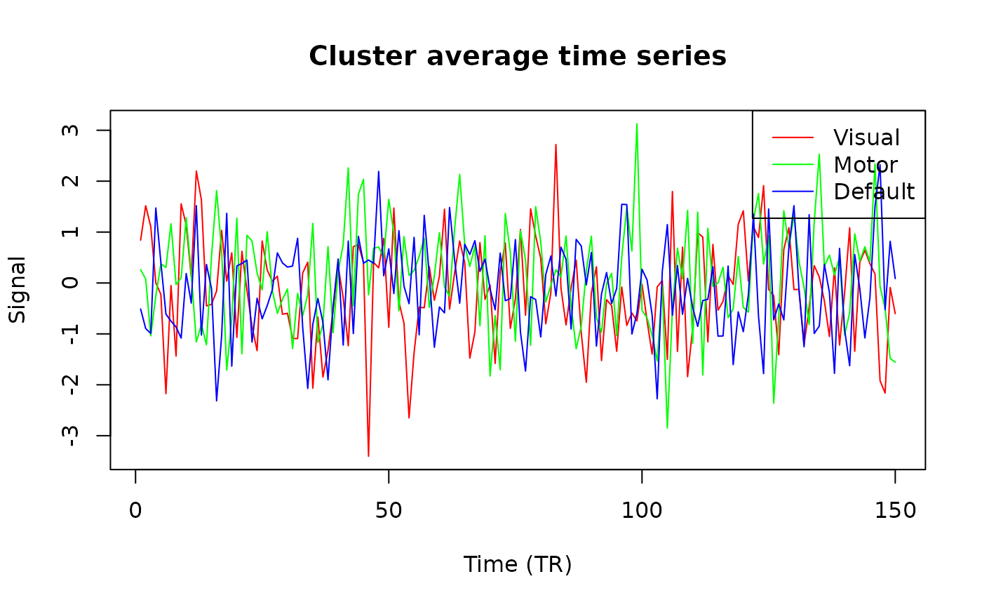

Memory Efficiency

The H5ClusterExperiment design provides several memory advantages:

Lazy loading: Data is only read when accessed
Partial reading: Can extract specific voxels or time ranges
Efficient storage: Similar signals are stored together

# Check file size
file_size_mb <- file.info(h5_file)$size / 1024^2
cat("HDF5 file size:", round(file_size_mb, 2), "MB\n")
#> HDF5 file size: 0.07 MB

# Memory usage of a specific extraction
object.size(ts_data) |> format(units = "Kb")
#> [1] "4.1 Kb"

Best Practices

Organize by similarity: Clusters should group functionally similar voxels
Use summary runs: For analyses that only need regional averages
Chunk appropriately: HDF5 chunking affects read performance
Close when done: Always close the HDF5 file handle

# Clean up
close(experiment)
unlink(h5_file)

Next Steps

See vignette("H5Neuro") for working with unclustered data
Explore LatentNeuroVec for dimensionality-reduced representations
Check the package documentation for advanced features

fmristore Package

2025-06-25