Volumes and vectors • neuroim2

library(neuroim2)

Two containers carry almost everything in neuroim2: NeuroVol for one 3D image and NeuroVec for a stack of them sharing a spatial frame. This article covers how to build them, take them apart, and put them back together.

anat <- demo_anatomy()
mask <- demo_mask()
bold <- demo_bold(n_time = 20)

class(anat)[1]
#> [1] "DenseNeuroVol"
class(bold)[1]
#> [1] "DenseNeuroVec"

demo_anatomy() and friends are shorthand this article set defines for the shipped example data; behind them are read_vol() for a 3D file, read_vec() for a 4D one, and simulate_fmri() for the functional series, which is simulated rather than read so its time courses have realistic temporal structure.

Note the classes: NeuroVol and NeuroVec are the generic constructors, and what you get back is a concrete implementation — DenseNeuroVol here, with the sparse and on-disk alternatives covered in vignette("large-data").

What survives an operation

These objects behave like arrays, but not every operation returns one that still knows where it is. The rule is worth learning early, because it decides when you have to reattach a space by hand.

Arithmetic and comparison preserve geometry — Arith, Compare and Logic group generics are all defined:

class(anat * 2)[1]
#> [1] "DenseNeuroVol"
class(anat > 100)[1]
#> [1] "LogicalNeuroVol"

Extraction deliberately does not. [ gives you plain R data:

dim(anat)
#> [1] 48 57 48
anat[24, 28, 24]
#> [1] 5033.67

class(anat[, , 24])[1]
#> [1] "matrix"
class(anat[anat > 100])[1]
#> [1] "numeric"

That is the right default — you usually want a matrix or a vector to compute on — but it means anything you build from extracted values has to be given a space again, which is the subject of the next section but one.

Masks

A comparison produces a LogicalNeuroVol — a mask that knows where it is:

brain <- anat > 100
class(brain)[1]
#> [1] "LogicalNeuroVol"
sum(brain)
#> [1] 32125

as.mask() is the explicit constructor, and takes either a logical volume or a set of indices:

from_logical <- as.mask(anat > 100)
from_indices <- as.mask(anat, which(anat > 6000))

c(brain = sum(from_logical), bright = sum(from_indices))
#>  brain bright 
#>  32125  23161

Masks index volumes directly, which is the usual way to pull out the voxels you care about:

vals <- anat[brain]

length(vals)
#> [1] 32125
mean(vals)
#> [1] 6472.492

op <- par(mfrow = c(1, 2), mar = c(1, 1, 2, 1))
image(anat[, , 24], main = "anat", col = gray.colors(256), axes = FALSE, asp = 1)
image(brain[, , 24], main = "anat > 100", col = gray.colors(2), axes = FALSE, asp = 1)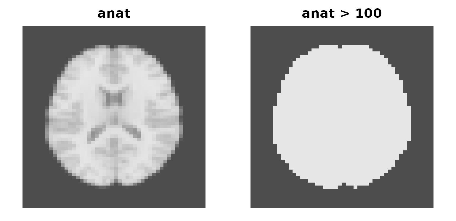

Two axial slices side by side: an anatomical slice and its binary mask.

A volume and the mask derived from it, same grid, same geometry.

par(op)

Building one by hand

A NeuroVol is an array plus a NeuroSpace:

set.seed(1)

sp <- NeuroSpace(dim = c(16L, 16L, 8L), spacing = c(2, 2, 2))
vol <- NeuroVol(array(rnorm(16 * 16 * 8), c(16, 16, 8)), sp)

vol
#> <DenseNeuroVol> [22.8 Kb] 
#> ── Spatial ───────────────────────────────────────────────────────────────────── 
#>   Dimensions    : 16 x 16 x 8
#>   Spacing       : 2 x 2 x 2 mm
#>   Origin        : 0, 0, 0
#>   Orientation   : RAS
#> ── Data ──────────────────────────────────────────────────────────────────────── 
#>   Range         : [-3.253, 3.810]

In practice you rarely write a space out. Arithmetic keeps the one it has, so the case that matters is rebuilding an image from values that have lost their geometry — anything that has been through [, as.matrix() or apply():

values <- as.array(anat)[]        # a plain numeric vector: no space
class(values)
#> [1] "array"

derived <- NeuroVol(values, space(anat))
identical(space(derived), space(anat))
#> [1] TRUE

The same for 4D, from either an array or a voxels-by-time matrix:

sp4 <- NeuroSpace(c(16L, 16L, 8L, 5L), spacing = c(2, 2, 2))
d <- rnorm(16 * 16 * 8 * 5)

v_arr <- NeuroVec(array(d, c(16, 16, 8, 5)), sp4)
v_mat <- NeuroVec(matrix(d, nrow = 16 * 16 * 8), sp4)

dim(v_arr)
#> [1] 16 16  8  5
all.equal(as.array(v_arr), as.array(v_mat))
#> [1] TRUE

Taking an object apart

A few ways, depending on what you want back.

A single volume, by position:

dim(bold[[3]])
#> [1] 64 64 25
class(bold[[3]])[1]
#> [1] "DenseNeuroVol"

A shorter series, keeping it 4D:

dim(sub_vector(bold, 1:5))
#> [1] 64 64 25  5

Every volume as a list, for iteration:

length(vols(bold))
#> [1] 20

For a 3D image the equivalent is slices() along the third axis, with slice() pulling one out as a NeuroSlice:

length(slices(anat))
#> [1] 48
class(slice(anat, 24, along = 3))[1]
#> [1] "NeuroSlice"

The matrix view

as.matrix() flattens a NeuroVec to voxels by time, which is the shape most modelling code wants:

mat <- as.matrix(bold)
dim(mat)
#> [1] 102400     20

Most of those rows are outside the brain and constant, so reduce over the mask and scatter the answers back. This masked form is the pattern you will use most often, and it is what the rest of these articles assume:

inside <- which(as.vector(mask) > 0)

ar1 <- numeric(nrow(mat))
ar1[inside] <- apply(mat[inside, ], 1, function(x) cor(x[-1], x[-length(x)]))

ar1_map <- NeuroVol(ar1, drop_dim(space(bold)))

c(voxels = nrow(mat), reduced = length(inside))
#>  voxels reduced 
#>  102400   29532
round(range(ar1[inside]), 3)
#> [1] -0.609  0.915

drop_dim() supplies the matching 3D space, which is what keeps the result aligned with its source. The reduction itself is a lag-1 autocorrelation — one number per voxel — and any vector-to-scalar function works in its place.

vectors() is the iterator form of the same idea, yielding one voxel time course at a time:

length(vectors(bold))
#> [1] 102400

Putting objects together

concat() stacks along time. Volumes become a series:

dim(concat(anat, anat, anat))
#> [1] 48 57 48  3

and series extend each other, which is how runs get joined:

run1 <- sub_vector(bold, 1:5)
run2 <- sub_vector(bold, 6:12)

dim(concat(run1, run2))
#> [1] 64 64 25 12

concat() takes the first argument’s NeuroSpace for the result and does not check that the others agree — a mismatched run is silently absorbed rather than rejected. Check before you concatenate:

identical(space(run1), space(run2))
#> [1] FALSE

split_blocks() is the inverse, cutting a concatenated series back into runs given a block label per timepoint:

joined <- concat(run1, run2)
blocks <- split_blocks(joined, rep(1:2, c(5, 7)))

length(blocks)
#> [1] 2
vapply(blocks, function(b) dim(b)[4], integer(1))
#> [1] 5 7

series() pulls one voxel’s time course directly, and series_roi() a whole region’s; regions, parcels and searchlights are the subject of vignette("regions-and-searchlights").

Dense and sparse

When a mask defines which voxels count, a sparse representation stores only those:

sparse <- as.sparse(bold, as.mask(mask))

class(sparse)[1]
#> [1] "SparseNeuroVec"
dim(sparse)
#> [1] 64 64 25 20

c(dense_MB = as.numeric(object.size(bold)) / 1e6,
  sparse_MB = as.numeric(object.size(sparse)) / 1e6)
#>  dense_MB sparse_MB 
#> 16.391504  5.684224

Dimensions are unchanged — sparsity is about storage, not shape — and as.dense() reverses it. read_vec(file, mask = ...) reads straight into the sparse form without materialising the dense one first.

class(as.dense(sparse))[1]
#> [1] "DenseNeuroVec"

When that trade is worth making, and the other backends available when data outgrows memory, is the subject of vignette("large-data").

Where to go next

vignette("reading-and-writing") — getting these objects to and from disk
vignette("regions-and-searchlights") — ROIs, parcels, searchlights
vignette("large-data") — sparse, mapped and file-backed storage

Reference: ?NeuroVol, ?NeuroVec, ?concat, ?sub_vector, ?as.mask.