GPCA at Scale and Special Cases

This vignette walks through the choices that matter once your data outgrows the defaults: which backend to pick, when to switch to a covariance-only fit, and how to project out-of-sample observations.

Backend selection

Method	Best for	Pros	Cons
`eigen`	Small / medium dense problems	Robust reference behaviour	Can be expensive at scale; very large sparse constraints may trigger truncated eigensolve via `maxeig`
`spectra`	Larger matrix-free solves	Lower memory than dense eigendecomp	Iterative behaviour can vary by conditioning
`randomized`	Wide (`p >> n`) low-rank workloads	Fast block GEMM / SpMM path	Approximation error depends on tuning
`deflation`	Few components, tight memory	Low memory footprint	Can converge slowly; monitor iteration warnings
`auto`	Default production usage	Picks among the dense and randomized paths	Heuristics may not be optimal for every regime

In practice, leave it on "auto" unless you have a reason to pin a backend.

Backends on the same problem

A small head-to-head on a dense problem so you can see how the singular values agree across paths:

set.seed(11)
n <- 150; p <- 60
X <- matrix(rnorm(n * p), n, p)

t_eig <- system.time(
  fit_eig <- genpca(X, ncomp = 8, method = "eigen",
                    preproc = multivarious::center())
)
t_rnd <- system.time(
  fit_rnd <- genpca(X, ncomp = 8, method = "randomized",
                    preproc = multivarious::center())
)
data.frame(method = c("eigen", "randomized"),
           elapsed = c(t_eig["elapsed"], t_rnd["elapsed"]),
           top_sv  = c(fit_eig$sdev[1], fit_rnd$sdev[1]))
#>       method elapsed   top_sv
#> 1      eigen   0.113 19.48896
#> 2 randomized   0.007 19.14753

Singular values from the eigen and randomized paths agree to plotting precision on this dense problem.

Sparse workflow (`spectra`)

The spectra backend uses an iterative C++ solver and is the right choice for large sparse problems. The chunk below is shown but not evaluated to keep the vignette fast; it is the pattern to copy:

set.seed(42)
X_sparse <- rsparsematrix(800, 300, density = 0.005)
fit_sp <- genpca(X_sparse, ncomp = 5, method = "spectra",
                 preproc = multivarious::pass(),
                 constraints_remedy = "ridge")
fit_sp$sdev

Covariance-only GPCA

When you already have the cross-product C = X' M X, genpca_cov() avoids touching the full data matrix:

set.seed(123)
n <- 100; p <- 15
X <- matrix(rnorm(n * p), n, p)
M <- diag(runif(n, 0.8, 1.2))
A <- diag(runif(p, 0.7, 1.3))
C <- t(X) %*% M %*% X
fit_cov <- genpca_cov(C, R = A, ncomp = 5, method = "gmd")
fit_cov$d
#> [1] 13.80217 12.42550 11.92054 11.15895 10.96560

Singular values from the covariance-only fit.

Out-of-sample projection

Fit on training rows, then project held-out observations into the same component space:

set.seed(7)
X <- matrix(rnorm(200 * 30), 200, 30)
fit <- genpca(X[1:150, ], ncomp = 4,
              preproc = multivarious::center())
scores_test <- multivarious::project(fit, X[151:200, ])
head(scores_test, 4)
#>            PC1        PC2        PC3        PC4
#> [1,] 1.9323426 -0.4080526 -0.1924407 -0.6673048
#> [2,] 0.3498745  0.6490485  0.2579339  0.9996621
#> [3,] 0.9590113  0.9305126 -1.4603670 -1.1496702
#> [4,] 0.1125973  1.0845757 -0.2493420 -1.2509707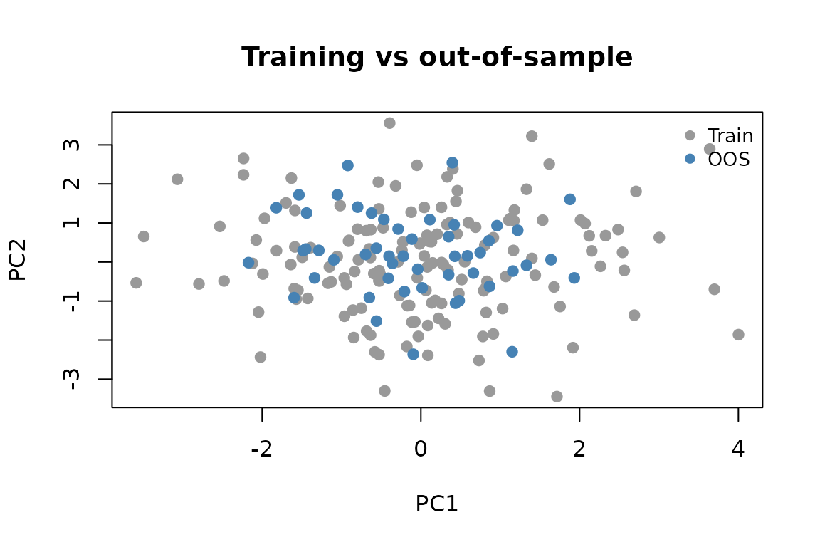

Training scores (grey) and out-of-sample scores (blue) projected into the same component space.

Performance tips

Keep data sparse when possible; avoid centering dense copies if you plan to use spectra. Use constraints_remedy = "ridge" for empirical metrics. For large problems, limit ncomp to what you truly need, and consider the covariance route when n is huge but p is moderate.

Where next

See vignette("gpca-metrics") for building metrics, and vignette("genpca") for a getting-started walkthrough.