fmristore: Efficient Storage for Neuroimaging Data
fmristore Package
2026-03-29
Source:vignettes/fmristore-overview.Rmd
fmristore-overview.RmdWhy fmristore?
A typical fMRI session produces 4D arrays with dimensions like 64 x
64 x 40 x 200 — over 32 million values per run. Load a few runs into R
and you quickly exhaust available memory. fmristore solves
this by storing neuroimaging data in HDF5 format: your data lives on
disk and is loaded on demand. The package also supports clustered
(parcellated) storage for ROI analyses, multi-run containers, and latent
decompositions for compression.
This vignette walks you through the main storage formats and when to use each one.
Quick Start: Choose Your Storage Format
                        Your Data
                       /    |    \
                      /     |     \
             Regular    Clustered   Multiple
             4D fMRI      Data     Brain Maps
                |          |           |
                v          v           v
           H5NeuroVec  H5Parcellated*  LabeledVolumeSet
Data Conversion Workflows
1. Converting neuroim2 ClusteredNeuroVec
The ClusteredNeuroVec class from neuroim2 stores
cluster-averaged time series data. Here’s the complete workflow:
# Create sample data
brain_dims <- c(10, 10, 5)
mask_data <- array(FALSE, brain_dims)
mask_data[3:7, 3:7, 2:4] <- TRUE
mask <- LogicalNeuroVol(mask_data, NeuroSpace(brain_dims))

# Define clusters
n_voxels <- sum(mask)
cluster_ids <- sample(1:3, n_voxels, replace = TRUE)
cvol <- ClusteredNeuroVol(mask, cluster_ids)

# Create time series (T x K matrix)
n_time <- 100
n_clusters <- 3
ts_data <- matrix(rnorm(n_time * n_clusters), nrow = n_time, ncol = n_clusters)

# Create ClusteredNeuroVec
cnvec <- ClusteredNeuroVec(x = ts_data, cvol = cvol)

# Convert to HDF5 (single scan by default)
h5_file <- tempfile(fileext = ".h5")
h5_scan <- as_h5(cnvec, file = h5_file, scan_name = "my_scan")

cat("Conversion result:\n")
#> Conversion result:
cat("  Input:", class(cnvec), "with", nrow(ts_data), "timepoints\n")
#>   Input: ClusteredNeuroVec with 100 timepoints
cat("  Output:", class(h5_scan), "\n")
#>   Output: H5ParcellatedScanSummary
cat("  Storage:", round(file.size(h5_file)/1024, 1), "KB\n")
#>   Storage: 21.9 KB

# Access the data
summary_matrix <- as.matrix(h5_scan)
cat("  Retrieved:", dim(summary_matrix)[1], "x", dim(summary_matrix)[2], "matrix\n")
#>   Retrieved: 100 x 3 matrix

close(h5_scan)
unlink(h5_file)
2. Converting Regular NeuroVec to HDF5
For standard 4D fMRI data:
# Create 4D fMRI data
fmri_dims <- c(10, 10, 5, 50)  # x, y, z, time
fmri_data <- array(rnorm(prod(fmri_dims)), dim = fmri_dims)
nvec <- NeuroVec(fmri_data, NeuroSpace(fmri_dims))

# Convert to HDF5-backed storage
h5_file <- tempfile(fileext = ".h5")
h5_nvec <- as_h5(nvec, file = h5_file)

cat("Regular NeuroVec conversion:\n")
#> Regular NeuroVec conversion:
cat("  Memory usage before:", format(object.size(nvec), units = "KB"), "\n")
#>   Memory usage before: 202.2 Kb
cat("  File size:", round(file.size(h5_file)/1024, 1), "KB\n")
#>   File size: 6 KB
cat("  Can access slices:", dim(h5_nvec[,,, 1:10]), "\n")
#>   Can access slices: 10 10 5 10

close(h5_nvec)
unlink(h5_file)
3. Creating Multi-Scan Experiments
When you have multiple runs with the same clustering:
# Create multiple ClusteredNeuroVec objects (e.g., multiple runs)
runs <- list()
for (i in 1:3) {
  ts <- matrix(rnorm(n_time * n_clusters), nrow = n_time, ncol = n_clusters)
  runs[[i]] <- ClusteredNeuroVec(x = ts, cvol = cvol)
}

# Option 1: Convert first run to multi-scan container
h5_file <- tempfile(fileext = ".h5")
h5_multi <- as_h5(runs[[1]],
                  file = h5_file,
                  scan_name = "run1",
                  as_multiscan = TRUE)

cat("Multi-scan container created:\n")
#> Multi-scan container created:
cat("  Type:", class(h5_multi), "\n")
#>   Type: H5ParcellatedMultiScan
cat("  Scans:", length(h5_multi@runs), "\n")
#>   Scans: 1

# Note: Currently, adding additional scans requires using write_dataset
# with the appropriate file management strategy

close(h5_multi)
unlink(h5_file)
Performance Comparison
Let’s compare different storage strategies:
# Create test data
dims <- c(64, 64, 40, 200)  # Realistic fMRI dimensions
n_voxels_total <- prod(dims[1:3])
n_voxels_brain <- round(n_voxels_total * 0.3)  # ~30% brain voxels

# Memory usage estimates
memory_full <- n_voxels_total * dims[4] * 8 / (1024^2)  # MB
memory_masked <- n_voxels_brain * dims[4] * 8 / (1024^2)  # MB
memory_clustered <- 100 * dims[4] * 8 / (1024^2)  # 100 clusters

sizes <- c(memory_full, memory_masked, memory_clustered)
names(sizes) <- c("Full volume", "Masked (30%)", "Clustered (100)")
cat("Compression ratio (full vs clustered):", round(memory_full / memory_clustered, 0), ":1\n")
#> Compression ratio (full vs clustered): 1638 :1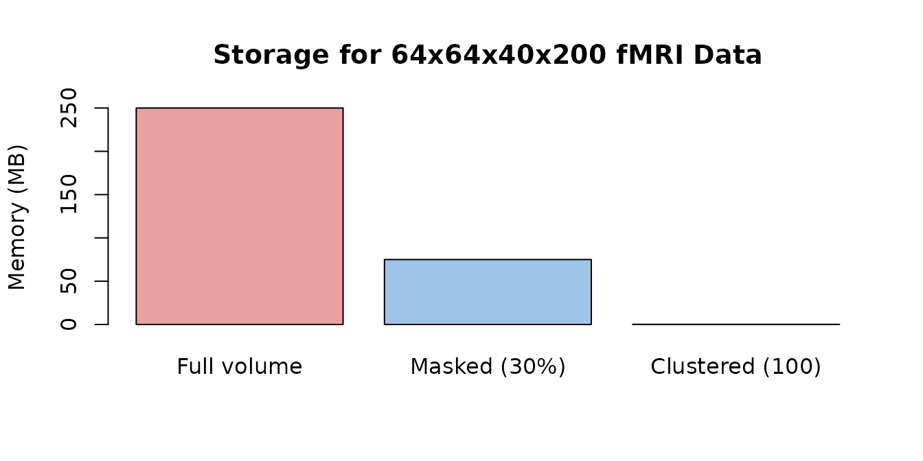
Memory requirements shrink dramatically with masking and clustering.
Best Practices
3. Data Access Patterns
# Efficient: Access contiguous slices from an H5NeuroVec
time_slice <- h5_nvec[, , , 1:10]  # Good

# Less efficient: Random access in time
random_times <- h5_nvec[, , , c(1, 50, 25, 75)]  # Slower

# For clustered data (H5ParcellatedScanSummary): get summary matrix once
summary_data <- as.matrix(h5_scan)  # Efficient
Common Use Cases
Use Case 1: Single Subject, Multiple Runs
# Typical fMRI experiment with multiple runs
n_runs <- 4
n_time_per_run <- 150

# Create clustering once (same for all runs)
mask <- LogicalNeuroVol(mask_data, NeuroSpace(brain_dims))
clusters <- ClusteredNeuroVol(mask, cluster_ids)

# Generate and save each run
for (run in 1:n_runs) {
  # Simulate run data
  ts <- matrix(rnorm(n_time_per_run * n_clusters),
               nrow = n_time_per_run, ncol = n_clusters)
  cnvec <- ClusteredNeuroVec(x = ts, cvol = cvol)

  # Save each run separately (simple approach)
  run_file <- tempfile(pattern = paste0("run", run, "_"), fileext = ".h5")
  h5_run <- as_h5(cnvec, file = run_file, scan_name = paste0("run", run))

  cat("Saved run", run, "as", class(h5_run), "\n")
  close(h5_run)
  unlink(run_file)  # Clean up for example
}
#> Saved run 1 as H5ParcellatedScanSummary
#> Saved run 2 as H5ParcellatedScanSummary
#> Saved run 3 as H5ParcellatedScanSummary
#> Saved run 4 as H5ParcellatedScanSummary
Use Case 2: Storing Subject Maps with LabeledVolumeSet
# Store activation maps from multiple subjects in a single HDF5 file
n_subjects <- 5
subject_data <- array(rnorm(prod(brain_dims) * n_subjects),
                      dim = c(brain_dims, n_subjects))
subject_vec <- NeuroVec(subject_data, NeuroSpace(c(brain_dims, n_subjects)))
subject_labels <- paste0("Subject_", sprintf("%02d", 1:n_subjects))

# Write to HDF5 with meaningful labels
h5_file <- tempfile(fileext = ".h5")
h5 <- write_labeled_vec(subject_vec, mask, subject_labels, file = h5_file)
h5$close_all()

# Load and access individual maps by name
lvs <- read_labeled_vec(h5_file)
cat("Stored", length(labels(lvs)), "subject maps:",
    paste(labels(lvs), collapse = ", "), "\n")
#> Stored 5 subject maps: Subject_01, Subject_02, Subject_03, Subject_04, Subject_05

subj1 <- lvs[["Subject_01"]]
cat("Subject_01 map dimensions:", paste(dim(subj1), collapse = "x"), "\n")
#> Subject_01 map dimensions: 10x10x5

close(lvs)
unlink(h5_file)
Use Case 3: Resting State Connectivity from Parcellated Data
# Store clustered resting-state time series and compute connectivity
rest_ts <- matrix(rnorm(n_time * n_clusters), nrow = n_time, ncol = n_clusters)

# Add shared signal to clusters 1 and 2 (simulating a network)
shared_signal <- rnorm(n_time, sd = 0.8)
rest_ts[, 1] <- rest_ts[, 1] + shared_signal
rest_ts[, 2] <- rest_ts[, 2] + shared_signal

# Save as parcellated scan via ClusteredNeuroVec
cnvec_rest <- ClusteredNeuroVec(x = rest_ts, cvol = cvol)
h5_file <- tempfile(fileext = ".h5")
h5_rest <- as_h5(cnvec_rest, file = h5_file, scan_name = "rest")

# Retrieve the cluster-average matrix and compute connectivity
rest_matrix <- as.matrix(h5_rest)
connectivity <- cor(rest_matrix)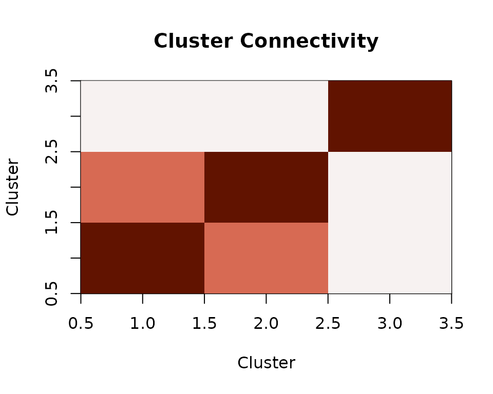
Inter-cluster connectivity from parcellated resting-state data.
Clusters 1 and 2 show elevated correlation because they share an underlying signal — exactly the kind of structure you would look for in resting-state connectivity analyses.
Advanced Features
Latent Representations
For data compression using basis decompositions:
n_vox <- 5000
n_tp <- 200
n_comp <- 20

basis <- matrix(rnorm(n_tp * n_comp), nrow = n_tp, ncol = n_comp)
loadings <- Matrix::Matrix(rnorm(n_vox * n_comp), nrow = n_vox, ncol = n_comp, sparse = TRUE)

lnv <- LatentNeuroVec(basis = basis,
                      loadings = loadings,
                      mask = mask,
                      space = NeuroSpace(c(brain_dims, n_tp)))

compression_ratio <- (n_vox * n_tp) / (n_tp * n_comp + n_vox * n_comp)
cat("Compression ratio:", round(compression_ratio, 1), ":1\n")
Working with Atlas Labels
For storing collections of named brain maps, see
vignette("LabeledVolumeSet"):
atlas_labels <- c("Visual", "Motor", "Default", "Attention", "Limbic")
n_labels <- length(atlas_labels)

atlas_data <- array(rnorm(prod(brain_dims) * n_labels),
                    dim = c(brain_dims, n_labels))
atlas_vec <- NeuroVec(atlas_data, NeuroSpace(c(brain_dims, n_labels)))

lvs_file <- tempfile(fileext = ".h5")
h5 <- write_labeled_vec(atlas_vec, mask, atlas_labels, file = lvs_file)
h5$close_all()

lvs <- read_labeled_vec(lvs_file)
labels(lvs)
close(lvs)
Troubleshooting
Common Issues and Solutions
-
Memory errors with large datasets
- Use HDF5-backed storage (
as_h5()) - Process data in chunks
- Use summary data instead of full voxel data
- Use HDF5-backed storage (
-
Slow data access
- Access contiguous slices when possible
- Use clustered/parcellated format for ROI analyses
- Consider caching frequently accessed data
-
File size concerns
- Enable compression:
compression = 4in write functions - Use summary data (
H5ParcellatedScanSummary) - Consider latent representations for compression
- Enable compression:
Next Steps
-
Basic HDF5 storage: See
vignette("H5Neuro") -
Clustered data details: See
vignette("H5ParcellatedScan") -
Multi-scan containers: See
vignette("H5ParcellatedMultiScan") -
Labeled volumes: See
vignette("LabeledVolumeSet")
Format Chooser
| Your data | Best format | Key function |
|---|---|---|
| Standard 4D fMRI | H5NeuroVec |
as_h5() |
| Clustered single scan | H5ParcellatedScanSummary |
as_h5() or
write_dataset()
|
| Multi-run clustered | H5ParcellatedMultiScan |
write_dataset() |
| Named brain maps | LabeledVolumeSet |
write_labeled_vec() |
| Compressed via PCA/ICA | LatentNeuroVec |
LatentNeuroVec() |