GazeWeave: Calibrated Item Information from Gaze Paths • eyesim

library(eyesim)
library(dplyr)
library(ggplot2)

The question GazeWeave answers

Experimental. GazeWeave is under active development. Its interface, defaults and result columns may change in future releases, so record the eyesim version alongside any results.

Suppose a participant studies a series of images and later recalls each one while looking at a blank screen. If recall reinstates the way the image was viewed, the recall gaze path should carry information about which image is being remembered. GazeWeave measures how much.

It treats this as an identification problem. For each recall path:

Compare it with every candidate. The candidates are a declared pool of study images, typically all items studied by the same participant (the contrast, set by contrast_on). Each candidate’s encoding path is compared with the recall path, giving a score for how well that candidate explains the recall.
Turn the scores into probabilities. The scores are converted into one probability per candidate. Calibration decides how far the scores are trusted, so that the probabilities are neither overconfident nor timid.
Ask how much the correct image gained. The result is the probability given to the correct image relative to the probability it had before gaze was considered.

Recall gaze is often shrunk and shifted relative to encoding gaze. You can declare a warp that corrects this before scoring; none is applied by default. Any warp, and the calibration, are learned from other trials, never from the recall being scored, and the same warp is applied to every candidate. Fitting on some trials and scoring others (cross-fitting) makes the final number an out-of-sample measure: a method that merely fits noise scores no better than zero on average.

GazeWeave does not combine several similarity dimensions into a profile, as MultiMatch does. It produces one number per recall.

Scoring in bits

The gain for the correct image is reported on a log scale:

$\mathrm{gaze\_info\_bits} = \log_2\frac{p(\mathrm{correct}\mid\mathrm{gaze})} {p(\mathrm{correct})}.$

Zero bits means that gaze did not improve on the candidate prior. One bit means that gaze doubled the probability assigned to the correct item relative to its prior. With $K$ equally likely candidates, the maximum is $\log_2 K$ . Negative values mean that gaze made the correct item less plausible.

gaze_info_bits is the sole primary endpoint. Coverage, spatial error, chronology, contraction, rank, and alignment stability are diagnostics nested within that score: they help explain it, but they are not further outcomes to test.

Choose an engine deliberately

The two engines differ in how they compare a recall path with a candidate.

Replay (engine = "replay") is directional. It models recall as a replay of the encoding path: recall fixations mostly step forward through the encoding sequence, sometimes restart at a new point, and sometimes fall on background locations unrelated to the candidate. A candidate’s score is the likelihood of the whole recall under this model, so evidence accumulates with every recall fixation. Use it for encoding-to-recall studies.
Transport (gaze_transport_cv()) is symmetric. It finds the best alignment between the two paths, matching fixations by position, penalizing disagreement in the order of neighbouring fixations, and allowing only part of each path to be matched. Use it when neither path has a privileged direction, or when several study presentations should inform each candidate.

There is no universal engine default. The common gaze_weave_cv() dispatcher accepts engine = "replay" or engine = "transport" and also infers the engine from gaze_replay_spec() or gaze_transport_spec(). Transport has a dedicated entry point because its episode identifiers and declared candidate priors are part of its estimand rather than optional plotting metadata.

The distinction affects interpretation. Replay’s braid contains posterior correspondence probabilities. Transport’s braid contains a regularized optimum; its diffuseness is partly controlled by numerical regularization and is not a posterior uncertainty statement.

A cross-fitted contraction example

The following paths differ by a known source-to-reference contraction and translation. Eight items keep the example compact while permitting an inner calibration split; scientific analyses should use more training items and predeclare the candidate pool.

make_path <- function(item) {
  anchor <- c(item * 2.5, (item %% 2) * 2.8)
  xy <- rbind(
    anchor,
    anchor + c(0.8, 1.1),
    anchor + c(1.7, -0.2),
    anchor + c(2.1, 0.7)
  )
  fixation_group(
    x = xy[, 1], y = xy[, 2],
    duration = c(1, 2, 1, 1), onset = c(0, 1, 3, 4)
  )
}

encoding_paths <- lapply(1:8, make_path)
recall_paths <- lapply(encoding_paths, function(path) {
  xy <- sweep(cbind(path$x, path$y), 2, c(0.4, -0.25), FUN = "-") / 0.75
  fixation_group(
    x = xy[, 1], y = xy[, 2],
    duration = path$duration * 1.5,
    onset = path$onset * 1.5
  )
})

encoding <- tibble(
  participant = "p1", image_id = 1:8, fixgroup = encoding_paths
)
recall <- tibble(
  participant = "p1", image_id = 1:8, fixgroup = recall_paths
)

The warp is learned only from training items and then applied identically to every candidate for a held-out path. Pair-specific free registration is not the default because it can rescue wrong templates.

replay_spec <- gaze_replay_spec(
  transition_grid = list(
    background = c(0.02, 0.08),
    restart = c(0.02, 0.08),
    advance = c(0.2, 0.4),
    background_stay = 0.9
  ),
  warp = gaze_warp_contraction(
    center = c(0, 0), translation = TRUE, fit_by = "participant"
  )
)

fit <- gaze_weave_cv(
  ref_tab = encoding,
  source_tab = recall,
  match_on = c("participant", "image_id"),
  contrast_on = "participant",
  split_on = c("participant", "image_id"),
  n_folds = 2,
  seed = 4,
  engine = "replay",
  spec = replay_spec
)

broom::tidy(fit)
#> # A tibble: 8 × 3
#>   participant image_id gaze_info_bits
#>   <chr>          <int>          <dbl>
#> 1 p1                 1           1.45
#> 2 p1                 2           1.47
#> 3 p1                 3           1.39
#> 4 p1                 4           1.39
#> 5 p1                 5           1.43
#> 6 p1                 6           1.43
#> 7 p1                 7           1.41
#> 8 p1                 8           1.45

tidy() returns only identifiers and gaze_info_bits. Candidate probability, log loss, rank, convergence, and fold columns are available through broom::tidy(fit, diagnostics = TRUE). The complete object retains candidate tables and the true-template alignment for audit and plotting.

Read the gaze braid

autoplot(
  fit,
  key = list(participant = "p1", image_id = 1),
  type = "overlay"
)

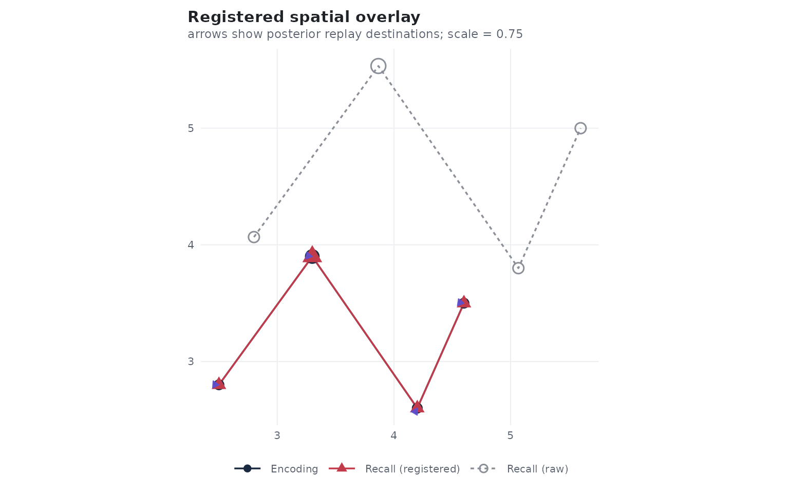
Encoding, raw recall, registered recall, and posterior replay destinations.

autoplot(
  fit,
  key = list(participant = "p1", image_id = 1),
  type = "braid"
)

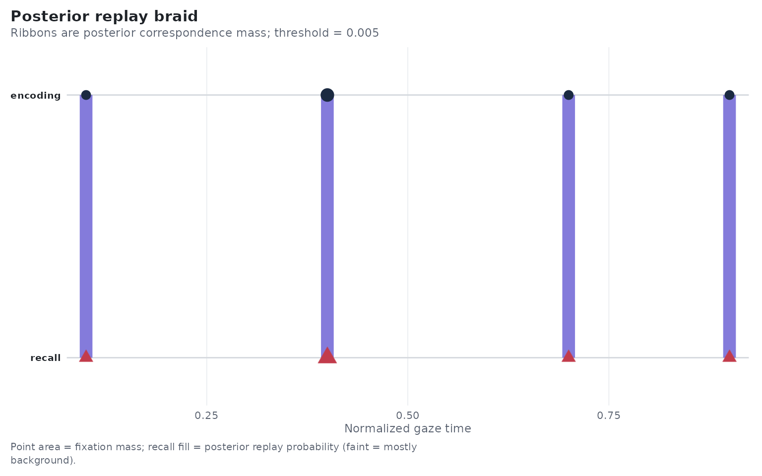
Replay posterior correspondence between encoding and recall fixations, in normalized time.

Parallel ribbons support local order preservation. Crossings can reflect chunk restarts or reordering. Faint recall time points support the background state. The diagnostic panel reports posterior replay coverage, background coverage, restart rate, and spatial RMSE. Those quantities explain the fitted replay but do not add up to gaze_info_bits, which is a contrast across candidate templates.

Fit symmetric Transport

Transport aligns two paths by finding the cheapest way to match the fixations of one with the fixations of the other, with each fixation weighted by its duration. Three things enter the cost:

Where. Matched fixations should be close in space.
Order. Each fixation’s next few fixations (two by default; see gaze_order_neighbours()) should be matched to fixations that are also among the next few in the other path; nearer neighbours count more. The order penalty is averaged over these local links and bounded, so its weight does not change with path length.
How much. Only part of each path needs to be matched. Which fixations take part is chosen separately from how they correspond. Rather than fixing the matched fraction, Transport integrates over a range of fractions under a fixed prior (coverage_prior), so the fractions that fit well dominate the result.

As with Replay, any warp is learned out of fold and applied identically to every candidate. The resulting correspondence is the best alignment under this cost. It is not a posterior probability that one fixation replays another, which is what Replay’s braid shows.

The example below turns each encoding path into two separate study presentations. The presentations are not concatenated: each candidate receives the mean of its two calibrated episode likelihoods. The one-presentation case uses exactly the same formula with weight one.

study <- expand.grid(
  participant = "p1",
  image_id = 1:8,
  presentation = 1:2,
  KEEP.OUT.ATTRS = FALSE,
  stringsAsFactors = FALSE
) %>%
  as_tibble()
study$fixgroup <- lapply(seq_len(nrow(study)), function(row) {
  path <- encoding_paths[[study$image_id[[row]]]]
  presentation <- study$presentation[[row]]
  fixation_group(
    x = path[["x"]] + 0.03 * (presentation - 1),
    y = path[["y"]] - 0.02 * (presentation - 1),
    duration = path[["duration"]],
    onset = path[["onset"]]
  )
})

transport_spec <- gaze_transport_spec(
  spatial = gaze_gaussian_mixture(c(0.5, 1), unit = "native"),
  warp = gaze_warp_contraction(
    center = c(0, 0), translation = TRUE, fit_by = "participant"
  ),
  # Lightweight deterministic controls for this executable vignette.
  coverage_nodes = 2,
  entropy_schedule = 0.03,
  maxit = 40,
  tolerance = 1e-3,
  projection_maxit = 300,
  projection_tolerance = 1e-7,
  backend = "optimized",
  reliability = "none"
)

The call declares the candidate stratum, outer split, episode identifier, and candidate prior. priorvar = NULL means a uniform design; a positive reference column supplies a nonuniform design prior. The compact solver controls above keep this vignette quick; a scientific protocol should freeze its coverage, solver, calibration, and reliability settings before outcomes are examined.

transport_fit <- gaze_transport_cv(
  ref_tab = study,
  source_tab = recall,
  match_on = c("participant", "image_id"),
  contrast_on = "participant",
  split_on = c("participant", "image_id"),
  episode_on = "presentation",
  priorvar = NULL,
  n_folds = 2,
  seed = 20260822,
  spec = transport_spec
)

broom::tidy(transport_fit)
#> # A tibble: 8 × 3
#>   participant image_id gaze_info_bits
#>   <chr>          <int>          <dbl>
#> 1 p1                 1        -0.0424
#> 2 p1                 2         1.94  
#> 3 p1                 3         1.99  
#> 4 p1                 4         0.306 
#> 5 p1                 5         0.999 
#> 6 p1                 6         1.91  
#> 7 p1                 7         1.77  
#> 8 p1                 8        -1.12

Default tidying exposes identifiers and gaze_info_bits only. Ask for the audit view when you need the explanatory fields:

transport_audit <- gaze_transport_result(
  transport_fit,
  key = list(participant = "p1", image_id = 1)
)

transport_audit$diagnostics[c(
  "matched_coverage", "spatial_rmse", "spatial_rmse_unit",
  "local_order_preservation", "contraction_scale", "template_rank",
  "episode_count", "episode_normalization", "solver_stability"
)]
#> $matched_coverage
#> [1] 0.4997673
#> 
#> $spatial_rmse
#> [1] 0.01803313
#> 
#> $spatial_rmse_unit
#> [1] "native_coordinate_units"
#> 
#> $local_order_preservation
#> [1] 0.9984414
#> 
#> $contraction_scale
#> [1] 0.7500076
#> 
#> $template_rank
#> [1] 2
#> 
#> $episode_count
#> [1] 2
#> 
#> $episode_normalization
#> [1] "fixed_equal_prior_likelihood_mixture"
#> 
#> $solver_stability
#> $solver_stability$all_converged
#> [1] TRUE
#> 
#> $solver_stability$backends
#> [1] "native_rcpparmadillo"
#> 
#> $solver_stability$maximum_stationarity
#> [1] 0.0009296708
#> 
#> $solver_stability$maximum_relative_objective_change
#> [1] 0.0001871428

Spatial RMSE is reported in the declared screen or spatial coordinate unit; a "native" specification is labelled native_coordinate_units. The nested episode table retains every equal weight, pair score, alignment diagnostic, backend, and convergence result.

The evidence panel displays the one inferential score. The other panels show a named episode so their provenance is visible; choosing another episode changes only the explanatory alignment panel, never the equal-prior score.

autoplot(
  transport_fit,
  key = list(participant = "p1", image_id = 1),
  type = "evidence"
)

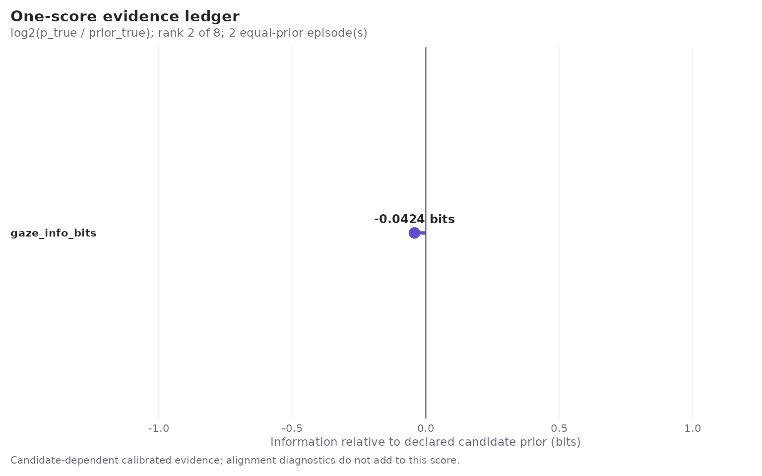
The one-score Transport evidence ledger.

autoplot(
  transport_fit,
  key = list(participant = "p1", image_id = 1),
  type = "braid",
  episode = transport_audit$diagnostics$episodes$episode[[1]]
)

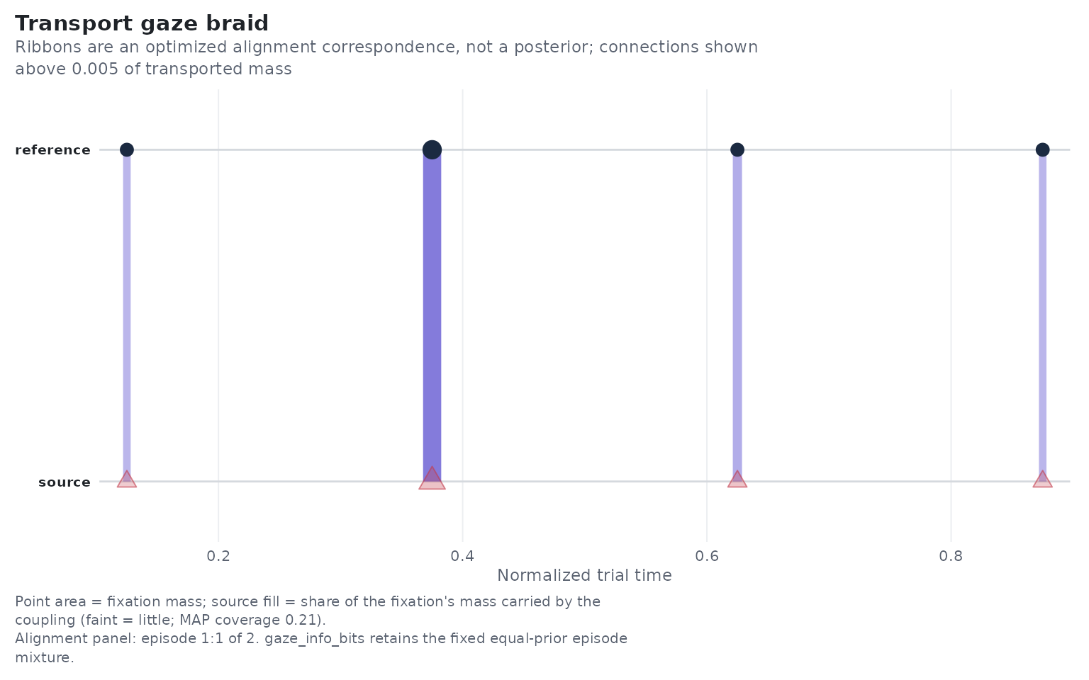
An optimized Transport correspondence, not a posterior probability.

Use type = "overlay", "raw_registered", or "diagnostics" for the registered spatial overlay, the raw-versus-registered path comparison, or the bounded diagnostic ledger. The public deterministic path fixtures and their MD5 manifest live under inst/validation/gaze-weave-transport-v3-golden in the source repository; the executable vignette above uses only generated paths. The v3 in those frozen paths identifies the development court, not a selectable method.

How scores become probabilities

Both engines convert candidate scores into probabilities the same way. This section describes the current model revision, revision = "2026.10", the default in gaze_replay_spec() and gaze_transport_spec(). The calibration controls are documented in ?gaze_calibration_control.

Replay scores. Replay observes each recall fixation once, with its position and its duration, and scores a candidate by the total log likelihood of the recall. Evidence therefore grows with the number of recall fixations, and there is no duration grid to choose. The earlier Replay revision "2026.08", which divided a duration-grid log likelihood by the number of grid bins, was retired in eyesim 0.3.0; the git tag gazeweave-2026.08-frozen reproduces it.

Temperature. Scores become probabilities through a softmax whose temperature sets how confident the probabilities are. One global temperature made sparse recalls overconfident and rich recalls underconfident, so each held-out row gets its own:

$T_i = T\left(\frac{\bar n}{n_i}\right)^\gamma ,$

where a row is one held-out recall, $n_i$ counts its evidence (Replay: the number of recall fixations; Transport: an effective count that equals the number of fixations when durations are equal and falls when a few long fixations dominate), and $\bar n$ is the geometric mean of that count over the calibration rows. $T$ and $\gamma \in [0, 1]$ are fitted only on training trials, by a second cross-validation nested inside each training set. The fit is regularized toward the declared candidate prior, that is, toward less confidence, never toward a fixed temperature. Calibration changes how confident the probabilities are; it never changes the reported ranking of candidates (template_rank, top1_credit).

Typicality. Some candidates match generic, centre-biased gaze well and would otherwise win by default. The typicality offset standardizes each candidate’s score against its scores on training recalls of other items. It is the default for Transport and opt-in for Replay. Adjusted scores are ranking scores, not normalized likelihoods, so do not read them as probabilities of the recall.

Small contrasts. Inner calibration needs at least twice as many items per contrast as calibration folds (four with the default two folds). With fewer, or when the inner folds cannot be built, the engine returns the declared prior and the row scores zero bits.

What the Transport courts support

Earlier internal experiments were labelled Transport v1, v2, and v3. Those were development names, never released APIs. The estimator formerly labelled v3 is now simply Transport; the older implementations have been removed. Version labels remain in internal and frozen validation provenance so the historical evidence stays auditable; they do not identify selectable methods.

The courts below ran the earlier Transport solver revision "2026.08", which was retired in eyesim 0.3.0 in favour of "2026.10" (see ?gaze_transport_spec); the git tag gazeweave-2026.08-frozen reproduces them.

The public frozen court passed representation, null calibration, chronology, coverage-refinement, registration, convergence, and perturbation gates. Reversal sensitivity stayed stable across the declared path-length range; 12-to-24-node coverage refinement changed pair energy by at most 9.65e-4 and candidate information by 4.60e-4 bits. Optimized and reference scores agree within 1e-8 on the differential court. On the frozen local runner, the 15-by-15 optimized pair took 8 ms versus 47 ms for the R reference, and the scope-matched 315-candidate fold took 13.955 seconds versus 830.849 seconds for the GW-14 implementation. These are local macOS arm64 measurements, not cross-platform guarantees.

The response-blind full-cohort study court also passed. P1-to-P4 Transport information was 0.28464 bits (crossed 95% interval 0.18206 to 0.38573), and the intact-minus-reversal/shuffle contrast was 0.05237 bits (0.00720 to 0.09536). Transport was effectively tied with the earlier development comparator then labelled v2, registered density, density sigma 80, and Replay on the common panel.

The exact frozen 0–3000 ms retrieval court did not support a retrieval claim. Transport had the largest response-blind point estimate, 0.02719 bits, but its crossed interval was -0.00305 to 0.05618 and principal comparator contrasts included zero. Adding Transport information to the held-out old-item response model changed predictive information by -0.01508 bits (-0.04322 to 0.00624). No algorithm, time window, calibration, subgroup, or saliency form was changed after behavior was opened.

The resulting product role is bounded: Transport is the symmetric explanatory alignment engine for order- and partial-replay questions. It is not a default retrieval predictor and is not known to outperform Replay, registered density, or MultiMatch generally. The complete public protocols, aggregate reports, and freeze receipts are under inst/validation in the source repository (they are not part of the CRAN package); trial-linked private outputs are excluded from Git and package artifacts.

Invariance contract

The recommended warp is participant/session contraction plus a calibration translation learned out of fold. Affine and pair-specific warps are not default nuisance corrections. Coordinate units, candidate pool, design prior, valid episode intersection, and episode count are part of the scientific estimand and must be reported.

Transport is invariant to candidate order, batch size, harmless time dilation, and fixation splitting that preserves the mass/edge representation within the frozen tolerances. It is deliberately sensitive to local-order reversal and coherent partial coverage. Results can fail or become uninterpretable when folds leak participant/item cells, candidate pools differ across conditions, coordinate units are undeclared, non-identity registration is fit on the scored pair, too few inner rows force identity calibration, or the solver does not converge. Treat those conditions as design or diagnostic failures, not as evidence of absent replay. New analyses should use gaze_transport_* for symmetric alignment or gaze_replay_* for the directional model and should treat gaze_info_bits as the primary endpoint.