Comparing Scanpaths with MultiMatch
Multimatch.RmdA single similarity number can hide important differences between scanpaths. Two people might fixate the same locations but in a completely different order, or follow the same trajectory but at different speeds. MultiMatch (Dewhurst et al., 2012) addresses this by evaluating scanpath similarity across five distinct dimensions:
| Dimension | What it captures |
|---|---|
| vector | Overall shape similarity of saccade vectors |
| direction | Angular similarity of saccade directions |
| length | Similarity of saccade amplitudes |
| position | Spatial proximity of corresponding fixations |
| duration | Similarity of fixation durations |
The eyesim implementation adds a sixth metric,
position_emd, based on the earth mover’s distance
between fixation locations. This captures distributional similarity that
is not order-dependent.
How do you compare two scanpaths?
Start by creating two fixation_group objects, convert
them to scanpath objects, and call
multi_match():
set.seed(1)

simulate_linear <- function(n) {
  fixation_group(
    x = cumsum(rnorm(n, mean = 50, sd = 10)),
    y = cumsum(rnorm(n, mean = 50, sd = 10)),
    duration = rpois(n, lambda = 200),
    onset = 1:n
  )
}

fg1 <- simulate_linear(10)
fg2 <- simulate_linear(12)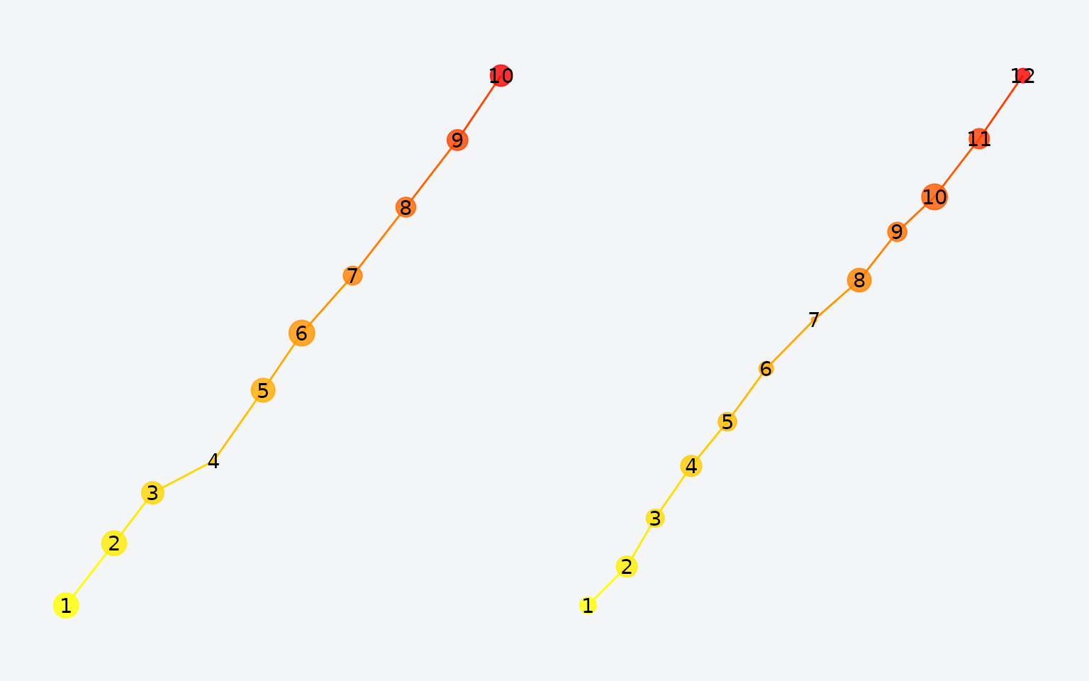
Two scanpaths generated from similar linear processes.
sp1 <- scanpath(fg1)
sp2 <- scanpath(fg2)
multi_match(sp1, sp2, screensize = c(500, 500))
#>       mm_vector    mm_direction       mm_length     mm_position     mm_duration
#>       0.9944381       0.9824906       0.9924735       0.8774572       0.9194313
#> mm_position_emd
#>       0.9646769
All metrics are high, consistent with the known similarity of the two scanpaths.
What happens when scanpaths differ structurally?
Let’s compare a linear scanpath against a zigzag pattern:
fg_zigzag <- fixation_group(
  x = cumsum(rep(50, 10)),
  y = cumsum(c(50, -50, 50, -50, 50, -50, 50, -50, 50, -50)),
  duration = rpois(10, lambda = 200),
  onset = 1:10
)

sp_linear <- scanpath(simulate_linear(10))
sp_zigzag <- scanpath(fg_zigzag)
multi_match(sp_linear, sp_zigzag, screensize = c(500, 500))
#>       mm_vector    mm_direction       mm_length     mm_position     mm_duration
#>       0.9914539       0.9671332       0.9912823       0.6570499       0.9350000
#> mm_position_emd
#>       0.6931491
Notice how the direction metric drops substantially — the zigzag and linear paths follow very different angular trajectories.
What do the metrics look like for random scanpaths?
To build intuition about each metric’s range and distribution, let’s simulate 500 pairs of random scanpaths and plot the results:
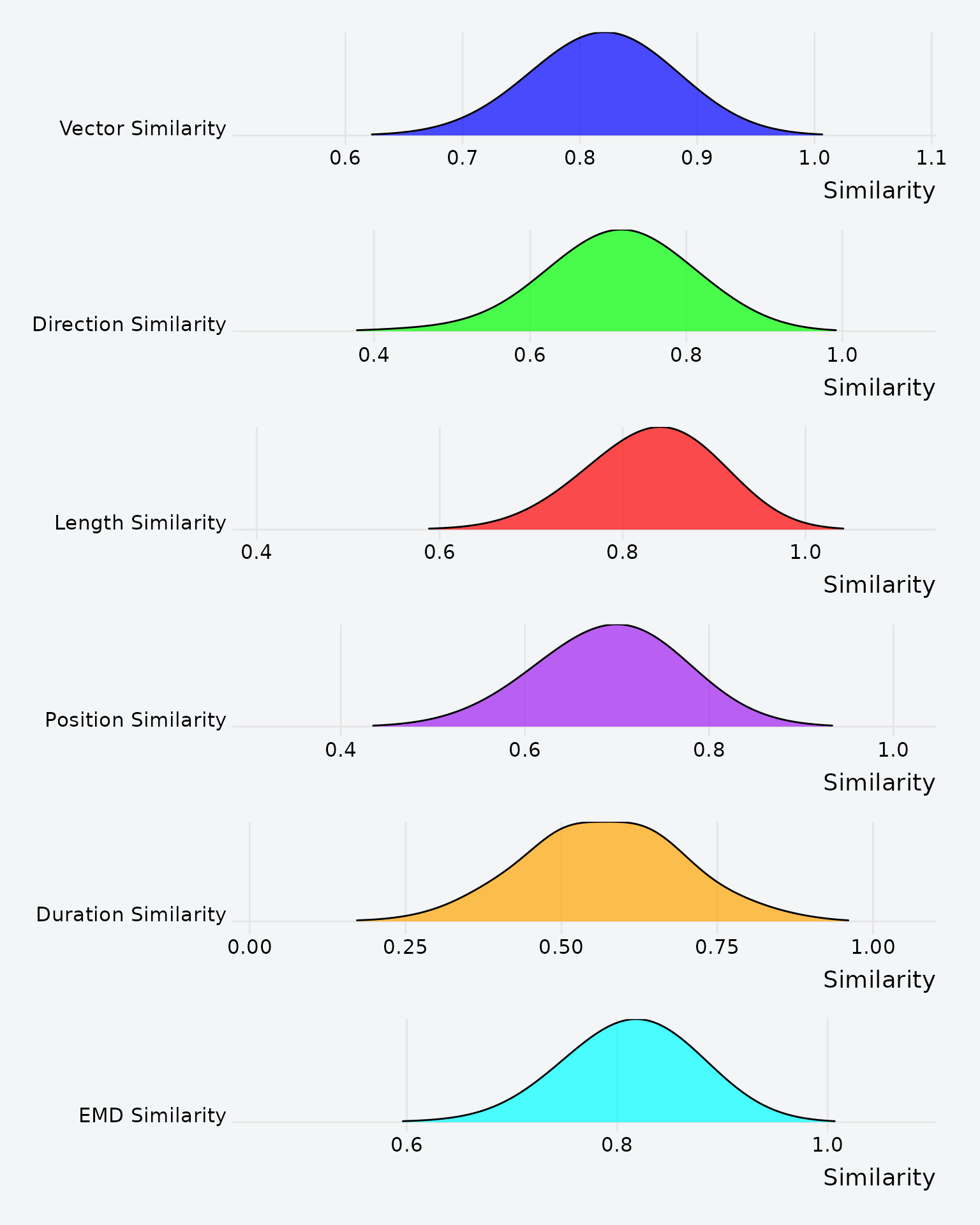
Distribution of each MultiMatch metric across 500 random scanpath pairs.
Each metric has a distinct baseline distribution. Direction similarity, for instance, clusters near 0.5 for random pairs, while position similarity is typically lower.
What do extreme matches look like?
Examining the highest- and lowest-scoring pairs for each metric gives concrete insight into what each dimension captures:
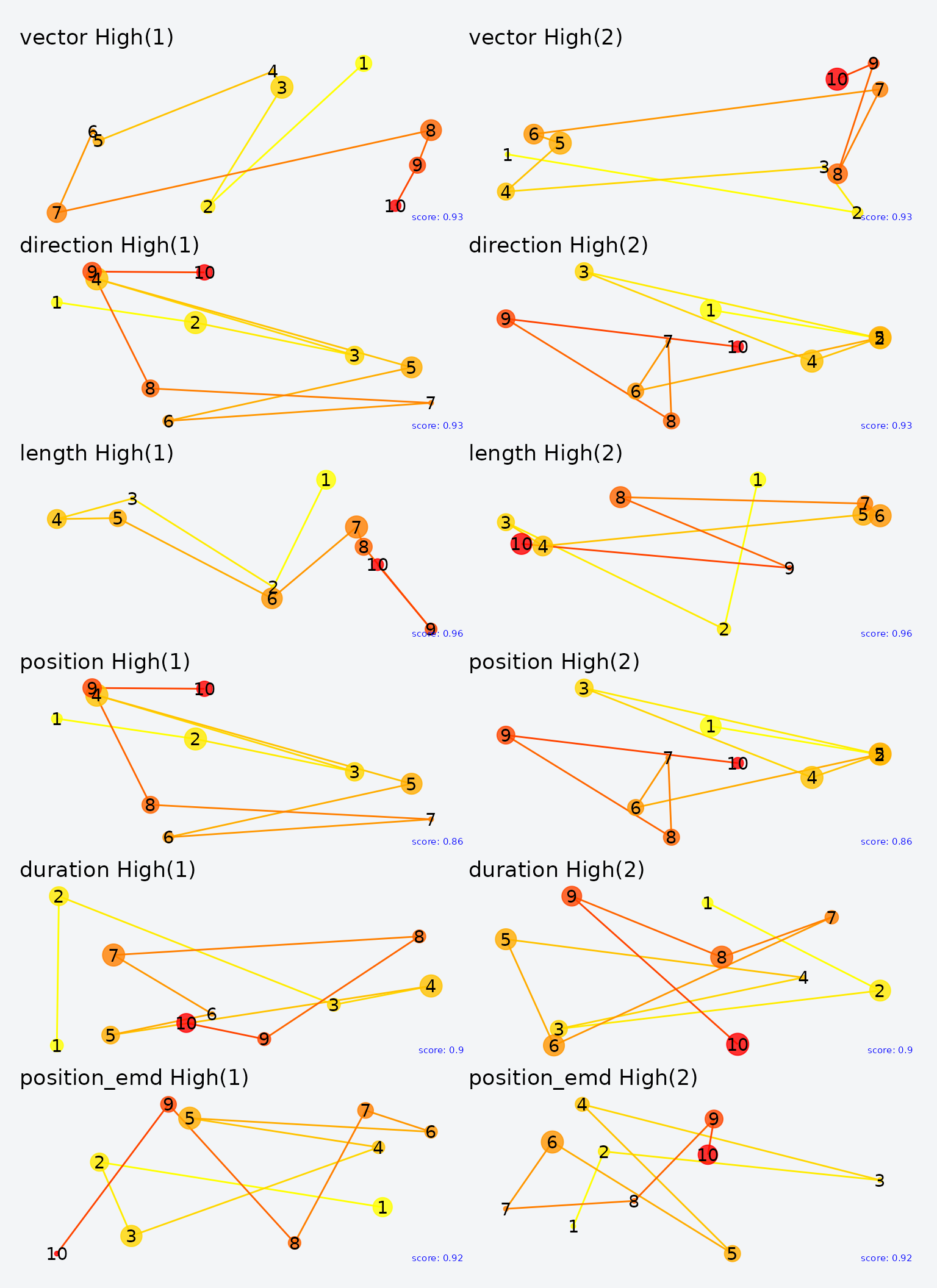
Highest-scoring pairs for each MultiMatch metric. Each row shows the two scanpaths that scored highest on that dimension.
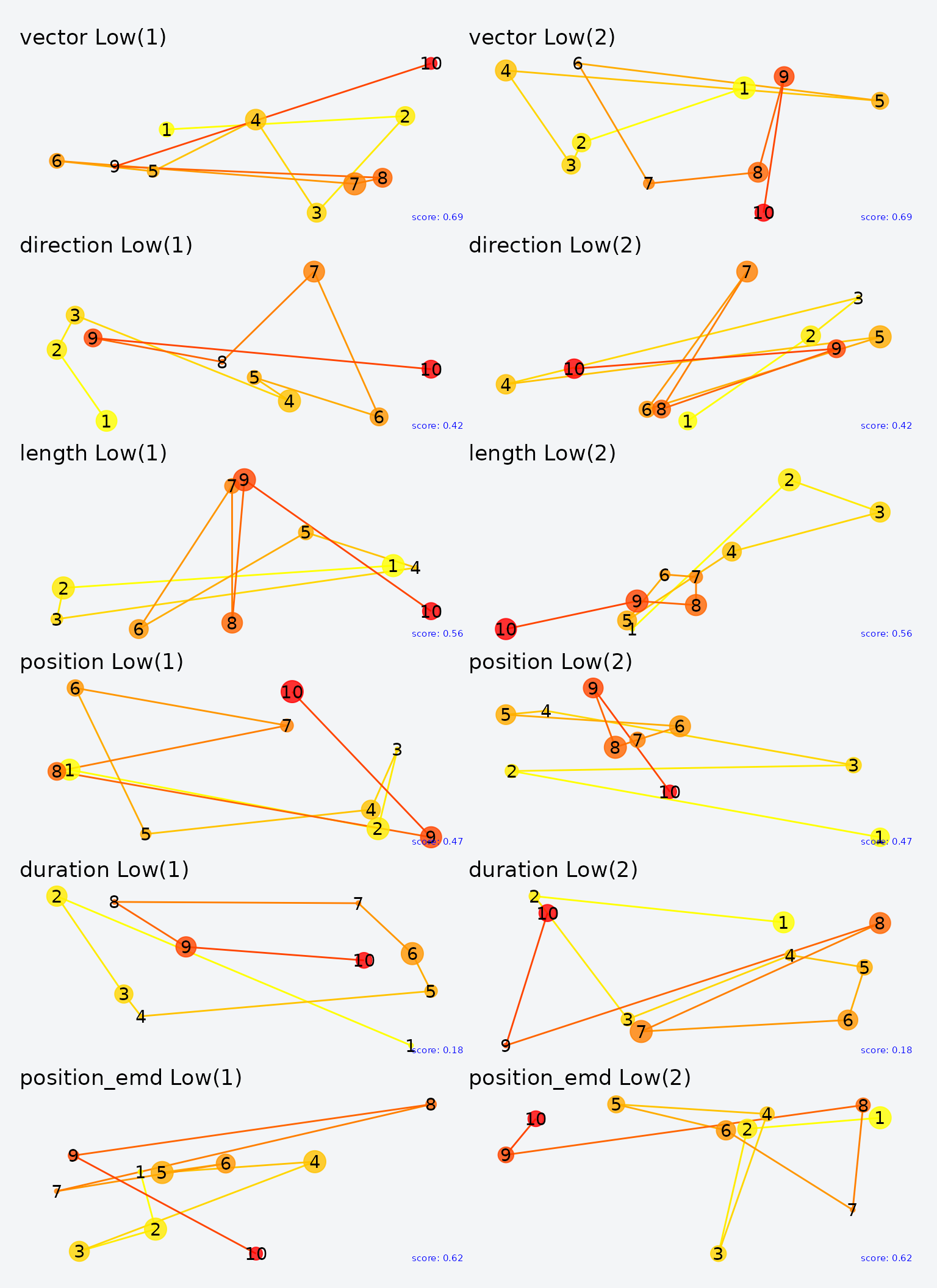
Lowest-scoring pairs for each metric.
How do transformations affect the metrics?
Understanding how each metric responds to spatial and temporal transformations helps you choose the right one for your research question.
Identity (perfect match)
set.seed(7)
fg <- fixation_group(runif(10) * 500, runif(10) * 500,
                     round(runif(10) * 10) + 1, 1:10)
multi_match(scanpath(fg), scanpath(fg), c(500, 500))
#>       mm_vector    mm_direction       mm_length     mm_position     mm_duration
#>               1               1               1               1               1
#> mm_position_emd
#>               1
All metrics are 1.0 — a scanpath is perfectly similar to itself.
Scaling
Scaling the coordinates by 0.5 preserves direction (relative angles are unchanged) but reduces position (absolute locations differ):
fg_scaled <- fg
fg_scaled$x <- fg_scaled$x * 0.5
fg_scaled$y <- fg_scaled$y * 0.5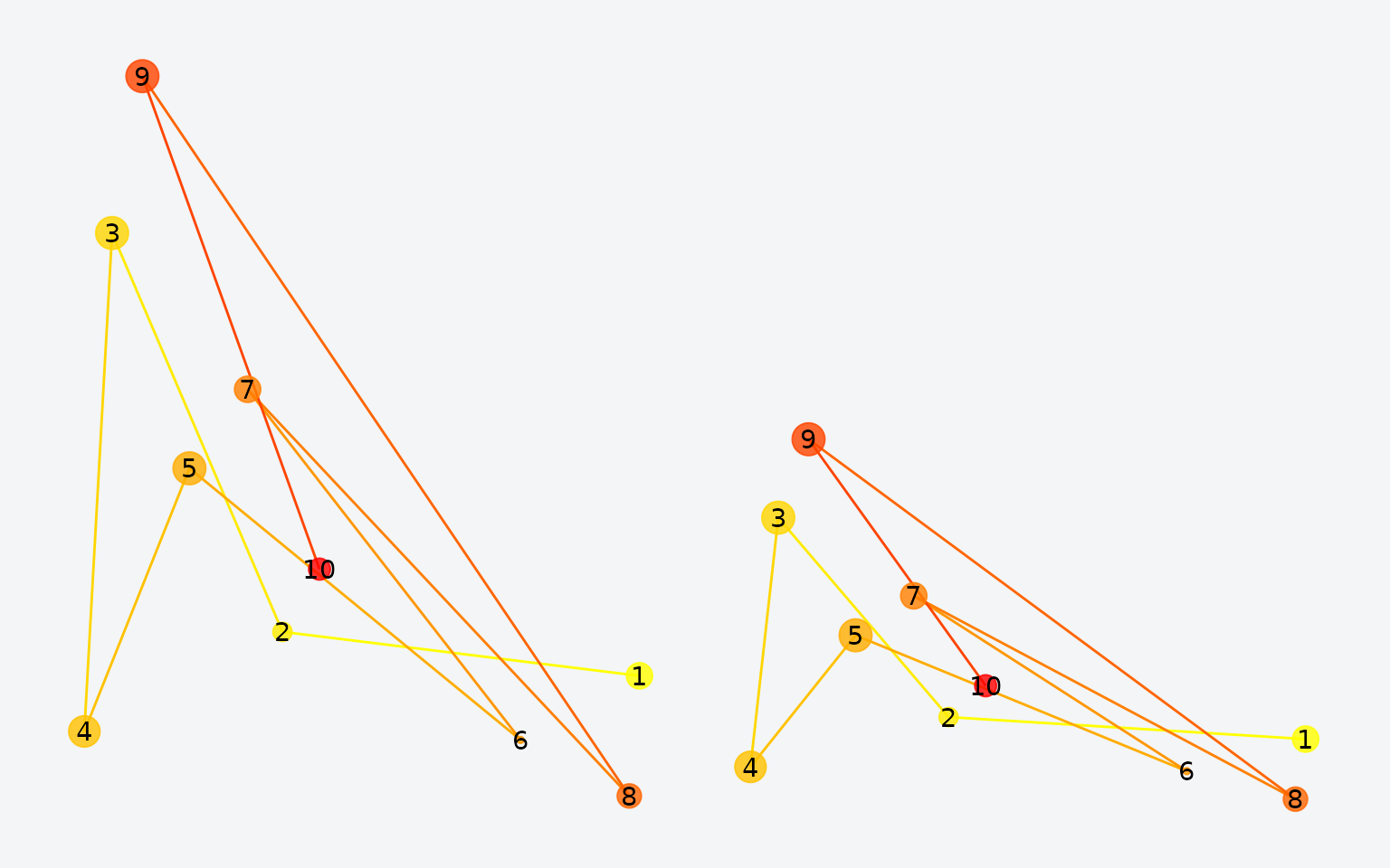
Original (left) vs. scaled (right) scanpath.
multi_match(scanpath(fg), scanpath(fg_scaled), c(500, 500))
#>       mm_vector    mm_direction       mm_length     mm_position     mm_duration
#>       0.8831983       1.0000000       0.7663966       0.7237247       1.0000000
#> mm_position_emd
#>       0.7575046
As expected, direction stays at 1.0, but position drops.
Shuffling fixation order
Keeping the same fixation locations but scrambling their order preserves position (and the EMD) while disrupting direction:
set.seed(3)
fg_shuffled <- fg
ord <- sample(nrow(fg_shuffled))
fg_shuffled$x <- fg_shuffled$x[ord]
fg_shuffled$y <- fg_shuffled$y[ord]
fg_shuffled$duration <- fg_shuffled$duration[ord]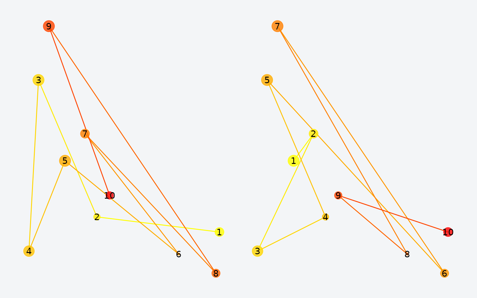
Original (left) vs. order-shuffled (right) scanpath. Same locations, different sequence.
multi_match(scanpath(fg), scanpath(fg_shuffled), c(500, 500))
#>       mm_vector    mm_direction       mm_length     mm_position     mm_duration
#>       0.8565614       0.7687388       0.7836460       0.7816592       0.6363636
#> mm_position_emd
#>       0.9710167
The position_emd remains high (same spatial distribution), while direction drops (the trajectory has changed).