Comparing Eye-Movement Patterns
eyesim.RmdWhen you study an image, you move your eyes to different locations in
a particular sequence. If you later see that same image during a memory
test, do you look at the same places? This kind of “eye-movement
reinstatement” is a powerful marker of memory, and eyesim
gives you the tools to measure it.
This vignette walks you through the core workflow: representing fixations, computing density maps, and measuring similarity between fixation patterns across experimental conditions.
How do you represent fixations?
A fixation_group holds a set of eye fixations — each
defined by an x/y screen position, an onset time (when the fixation
began), and a duration (how long the eye stayed there). You can create
one directly:
fg <- fixation_group(
  x = c(-100, 0, 100),
  y = c(0, 100, 0),
  onset = c(0, 10, 60),
  duration = c(10, 50, 100)
)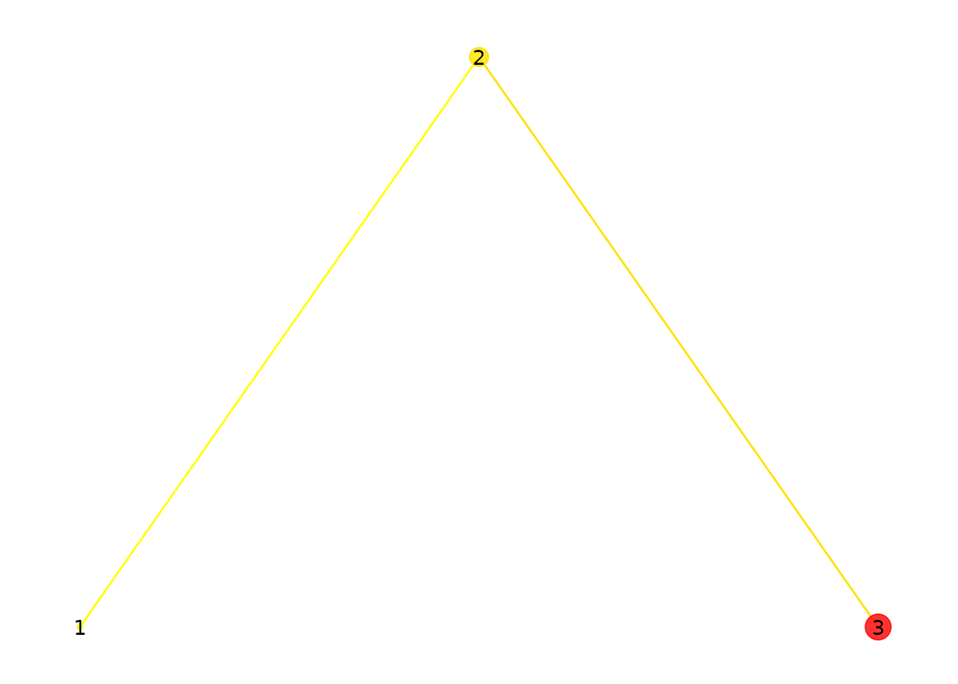
Three fixations. Point size reflects duration; color reflects onset time (yellow = early, red = late).
Point size shows how long each fixation lasted. Color indicates when it occurred: yellow for early fixations, red for later ones.
Here is a more realistic group with 25 randomly placed fixations:
set.seed(42)
fg <- fixation_group(
  x = runif(25, 0, 100),
  y = runif(25, 0, 100),
  onset = cumsum(runif(25, 0, 100)),
  duration = runif(25, 50, 300)
)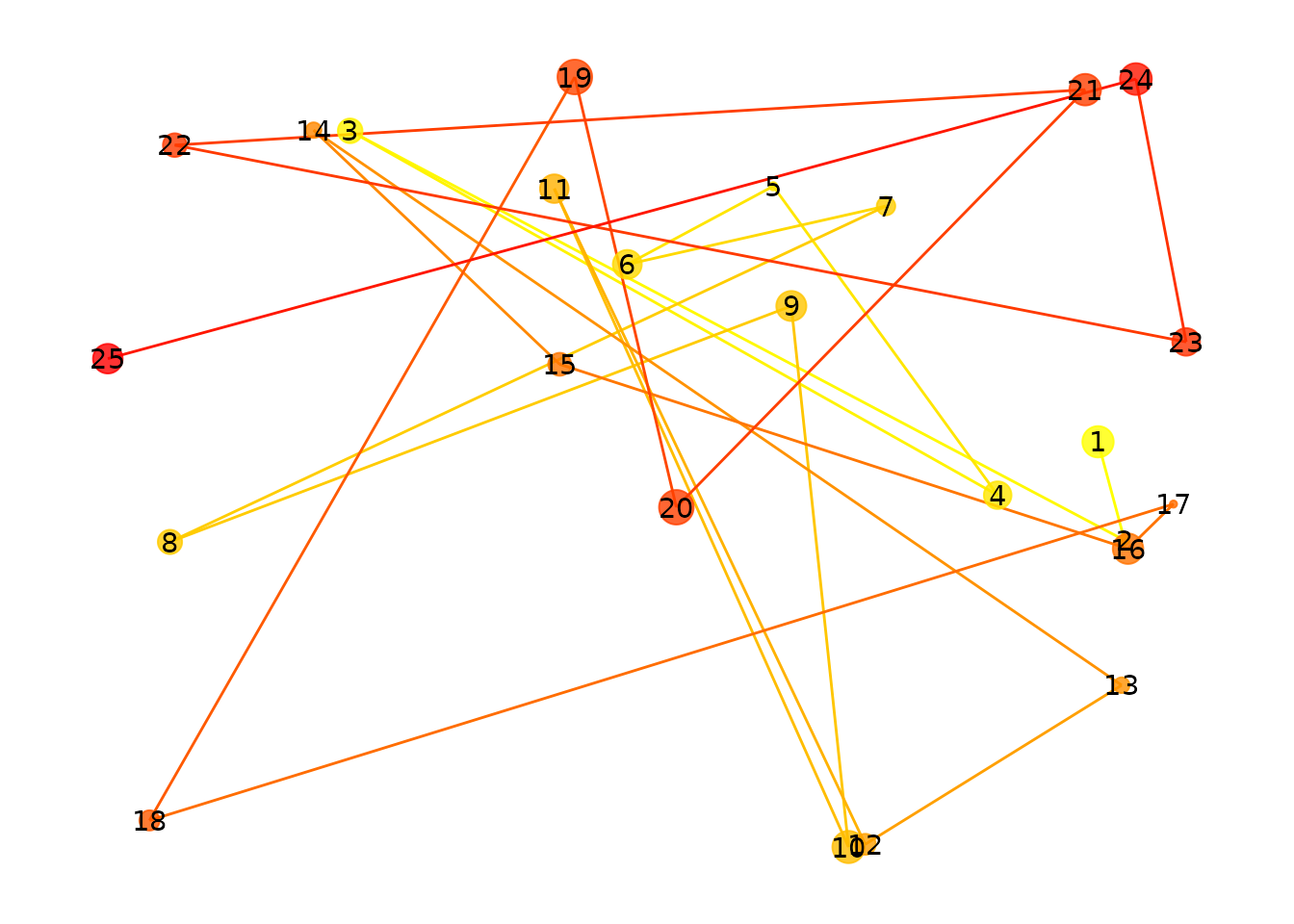
25 randomly placed fixations.
How do you visualize fixation density?
Individual points can be hard to interpret. Density maps show you
where fixations cluster. The plot() method supports several
display styles:
p1 <- plot(fg, typ = "contour", xlim = c(-10, 110), ylim = c(-10, 110), bandwidth = 35)
p2 <- plot(fg, typ = "raster", xlim = c(-10, 110), ylim = c(-10, 110), bandwidth = 35)
p3 <- plot(fg, typ = "filled_contour", xlim = c(-10, 110), ylim = c(-10, 110), bandwidth = 35)
p1 + p2 + p3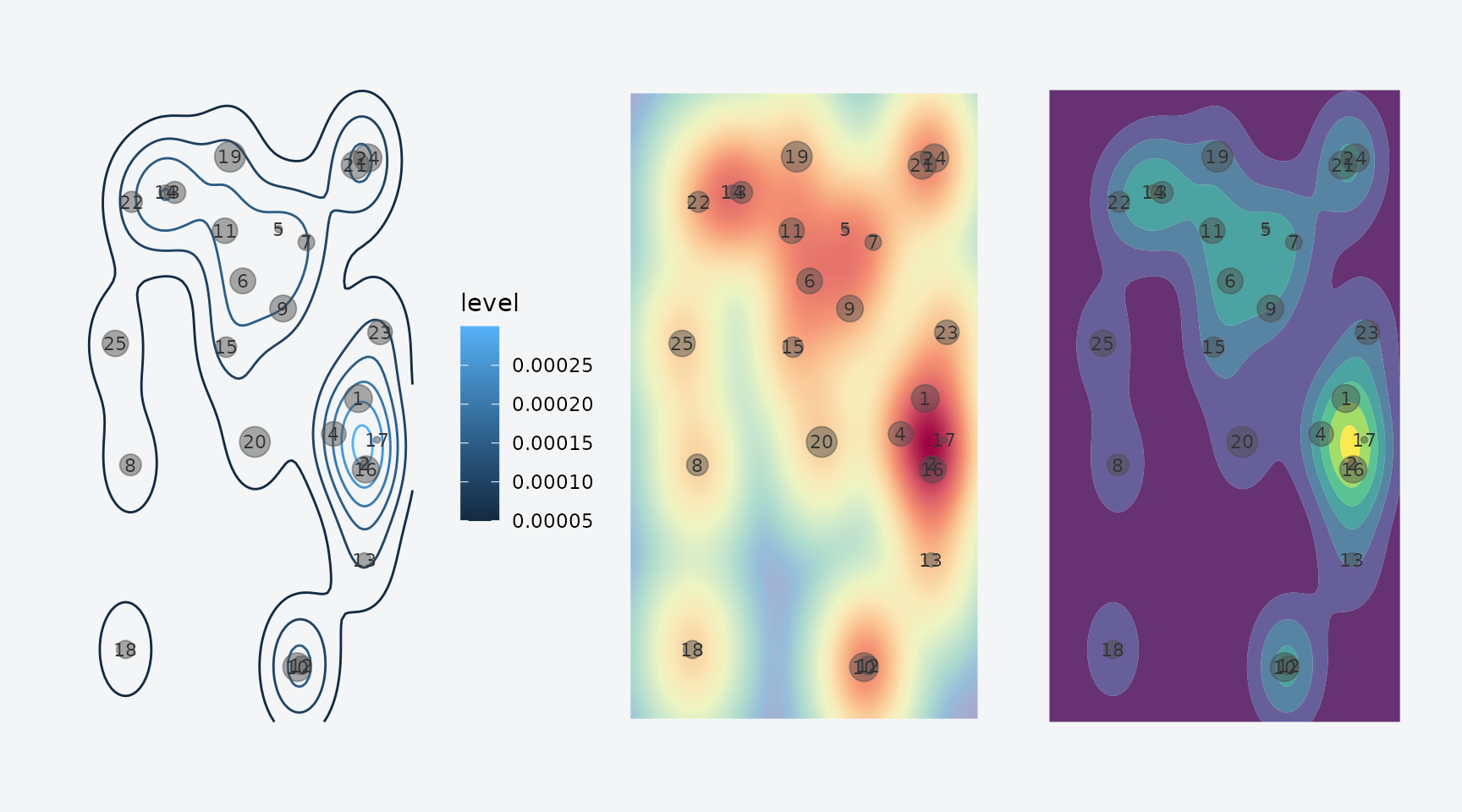
Three density visualizations: contour, raster, and filled contour.
The bandwidth parameter controls the smoothing level.
Higher values blur out fine detail and emphasize broad patterns:
p1 <- plot(fg, typ = "filled_contour", xlim = c(-10, 110), ylim = c(-10, 110), bandwidth = 20)
p2 <- plot(fg, typ = "filled_contour", xlim = c(-10, 110), ylim = c(-10, 110), bandwidth = 60)
p3 <- plot(fg, typ = "filled_contour", xlim = c(-10, 110), ylim = c(-10, 110), bandwidth = 100)
p1 + p2 + p3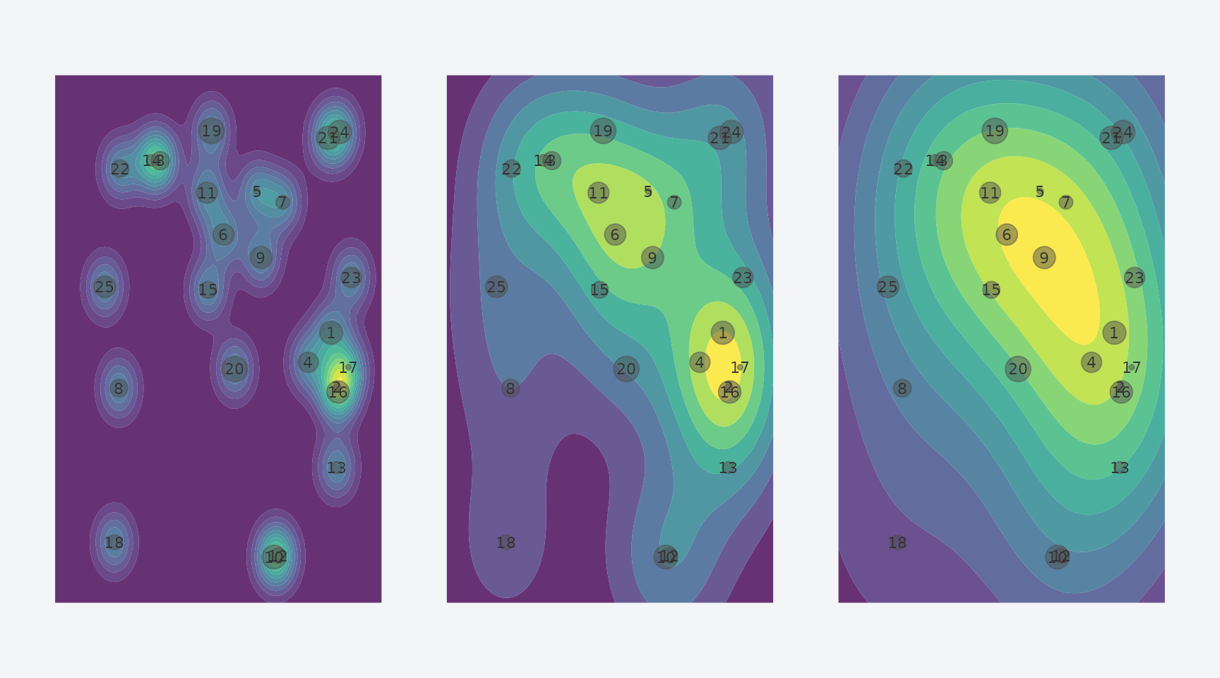
Effect of bandwidth: narrow (20), medium (60), and wide (100).
How do you compare two fixation patterns?
To quantify how similar two fixation patterns are, convert them to
eye_density maps and call similarity(). Here
we create two patterns that share roughly half their fixation
locations:
set.seed(123)
x_shared <- runif(12, 0, 100)
y_shared <- runif(12, 0, 100)

fg1 <- fixation_group(
  x = c(x_shared, runif(13, 0, 100)),
  y = c(y_shared, runif(13, 0, 100)),
  onset = cumsum(runif(25, 0, 100)),
  duration = runif(25, 50, 300)
)

fg2 <- fixation_group(
  x = c(x_shared, runif(13, 0, 100)),
  y = c(y_shared, runif(13, 0, 100)),
  onset = cumsum(runif(25, 0, 100)),
  duration = runif(25, 50, 300)
)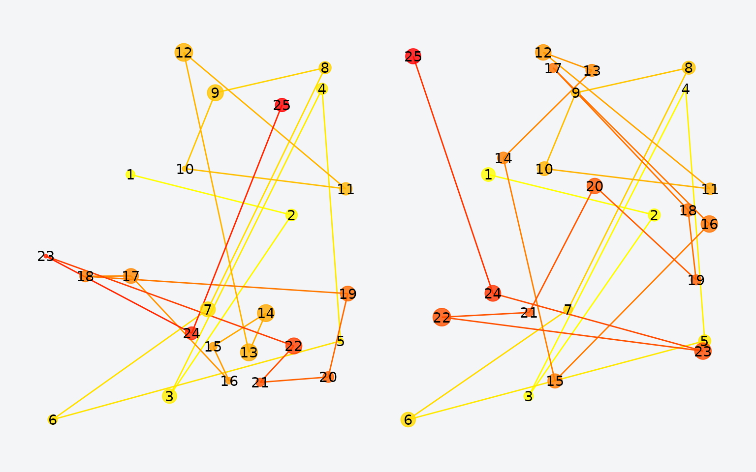
Two fixation patterns sharing roughly half their locations.
Now convert to density maps and compute their similarity:
ed1 <- eye_density(fg1, sigma = 50, xbounds = c(0, 100), ybounds = c(0, 100))
ed2 <- eye_density(fg2, sigma = 50, xbounds = c(0, 100), ybounds = c(0, 100))
similarity(ed1, ed2)
#> [1] 0.7760392
The default metric is the Pearson correlation. Several alternatives are available:
methods <- c("pearson", "spearman", "fisherz", "cosine", "l1", "jaccard", "dcov")
results <- sapply(methods, function(m) similarity(ed1, ed2, method = m))
data.frame(method = methods, similarity = round(unlist(results), 4))
#>            method similarity
#> pearson   pearson     0.7760
#> spearman spearman     0.7714
#> fisherz   fisherz     1.0353
#> cosine     cosine     0.9934
#> l1             l1     0.9484
#> jaccard   jaccard     0.9869
#> dcov         dcov     0.7293
How do you analyze a full experiment?
In a typical memory study, participants view images during encoding and again during retrieval. You want to compare fixation patterns between these phases for the same image and control for non-specific similarity.
Let’s simulate a small experiment: 3 participants, 20 images, encoding + retrieval.
head(df)
#>          x        y     onset duration image    phase participant
#> 1 11.37817 50.54517  62.07862 197.0510  img1 encoding          s1
#> 2 68.42647 19.38365 235.32139 204.0351  img1 encoding          s1
#> 3 99.25088 63.69041 373.98848 263.6462  img1 encoding          s1
#> 4 53.49936 68.78001 539.99684 112.1470  img1 encoding          s1
#> 5 96.66141 64.01908 642.50973 233.1542  img1 encoding          s1
#> 6 67.14276 35.78854 693.41893 307.2941  img1 encoding          s1
cat("Rows:", nrow(df),
    " | Participants:", length(unique(df$participant)),
    " | Images:", length(unique(df$image)))
#> Rows: 783  | Participants: 3  | Images: 20
Wrap the raw data in an eye_table, which groups
fixations by the variables that define your experimental design:
eyetab <- eye_table("x", "y", "duration", "onset",
                    groupvar = c("participant", "phase", "image"),
                    data = df)
eyetab
#> Eye table: 120 groups, 783 total fixations
#>   origin: (640, 640)
#> # A tibble: 120 × 4
#>    participant phase    image fixgroup
#>    <chr>       <chr>    <chr> <list>
#>  1 s1          encoding img1  <fxtn_grp [10 × 6]>
#>  2 s1          encoding img10 <fxtn_grp [4 × 6]>
#>  3 s1          encoding img11 <fxtn_grp [3 × 6]>
#>  4 s1          encoding img12 <fxtn_grp [10 × 6]>
#>  5 s1          encoding img13 <fxtn_grp [10 × 6]>
#>  6 s1          encoding img14 <fxtn_grp [4 × 6]>
#>  7 s1          encoding img15 <fxtn_grp [10 × 6]>
#>  8 s1          encoding img16 <fxtn_grp [7 × 6]>
#>  9 s1          encoding img17 <fxtn_grp [3 × 6]>
#> 10 s1          encoding img18 <fxtn_grp [4 × 6]>
#> # ℹ 110 more rows
Computing density maps by group
density_by() computes a density map for every
combination of your grouping variables:
eyedens <- density_by(eyetab,
                      groups = c("phase", "image", "participant"),
                      sigma = 100,
                      xbounds = c(0, 100), ybounds = c(0, 100))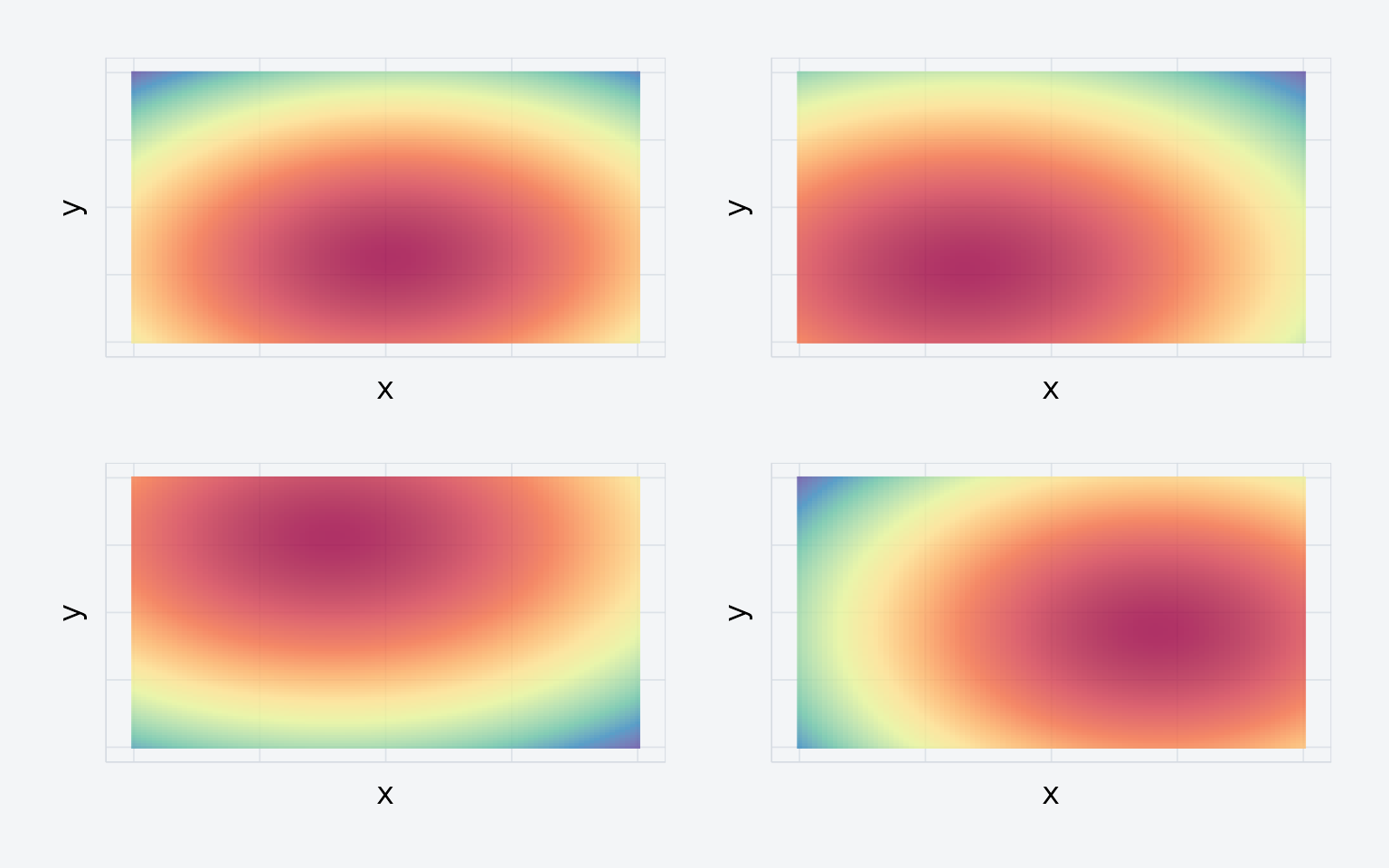
Four density maps from the simulated experiment.
eyedens
#> # A tibble: 120 × 5
#>    phase    image participant fixgroup            density
#>    <chr>    <chr> <chr>       <list>              <list>
#>  1 encoding img1  s1          <fxtn_grp [10 × 6]> <ey_dnsty [5]>
#>  2 encoding img1  s2          <fxtn_grp [8 × 6]>  <ey_dnsty [5]>
#>  3 encoding img1  s3          <fxtn_grp [8 × 6]>  <ey_dnsty [5]>
#>  4 encoding img10 s1          <fxtn_grp [4 × 6]>  <ey_dnsty [5]>
#>  5 encoding img10 s2          <fxtn_grp [4 × 6]>  <ey_dnsty [5]>
#>  6 encoding img10 s3          <fxtn_grp [8 × 6]>  <ey_dnsty [5]>
#>  7 encoding img11 s1          <fxtn_grp [3 × 6]>  <ey_dnsty [5]>
#>  8 encoding img11 s2          <fxtn_grp [3 × 6]>  <ey_dnsty [5]>
#>  9 encoding img11 s3          <fxtn_grp [9 × 6]>  <ey_dnsty [5]>
#> 10 encoding img12 s1          <fxtn_grp [10 × 6]> <ey_dnsty [5]>
#> # ℹ 110 more rows
Template similarity analysis
template_similarity() compares each retrieval density
map to its matched encoding density map. It estimates a baseline by
permuting image labels and reports the corrected difference:
set.seed(1234)
enc_dens <- eyedens %>% filter(phase == "encoding")
ret_dens <- eyedens %>% filter(phase == "retrieval")

simres <- template_similarity(enc_dens, ret_dens,
                              match_on = "image",
                              method = "fisherz",
                              permutations = 50)
The result includes three key columns:
-
eye_sim— raw similarity between matched pairs -
perm_sim— average similarity across non-matching pairs (baseline) -
eye_sim_diff— the corrected score (raw minus baseline)
Since our data is random, there should be no true reinstatement:
t.test(simres$eye_sim_diff)
#>
#>  One Sample t-test
#>
#> data:  simres$eye_sim_diff
#> t = 0.78502, df = 59, p-value = 0.4356
#> alternative hypothesis: true mean is not equal to 0
#> 95 percent confidence interval:
#>  -0.1021582  0.2340630
#> sample estimates:
#>  mean of x
#> 0.06595242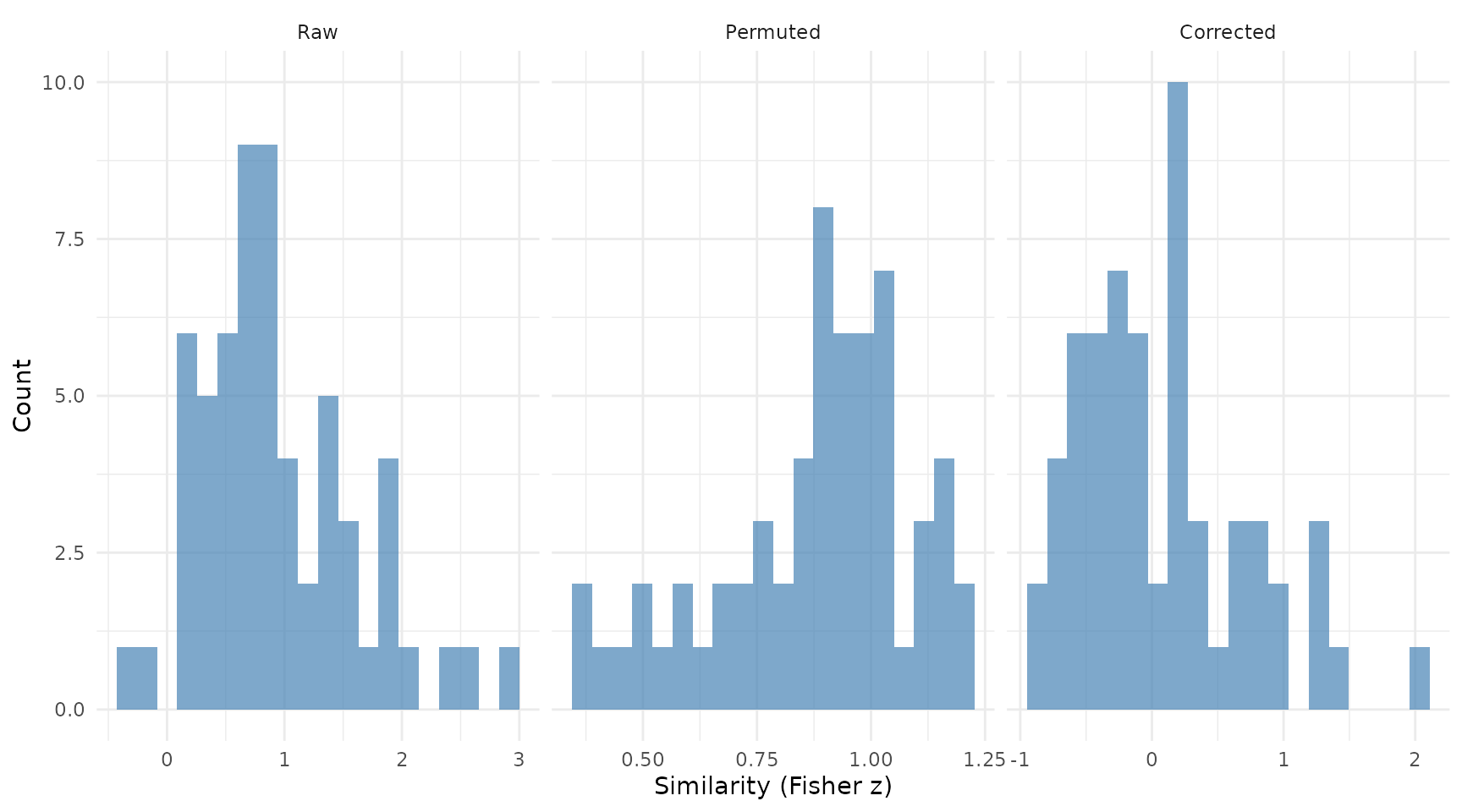
Distribution of raw, permuted, and corrected similarity scores.
As expected, the corrected similarity is centered near zero.
A note on units. With
method = "fisherz", all similarity values are Fisher z
scores (atanh of Pearson r). Convert back to correlations with
tanh() if desired. With method = "pearson" or
"spearman", values are correlations directly.
A note on permutations. The
permutations argument is an upper bound. If fewer
non-matching candidates are available, eyesim uses all of
them exhaustively.
What about multiscale analysis?
Choosing a single bandwidth is somewhat arbitrary. You can compute density at multiple scales by passing a vector of sigma values:
eyedens_multi <- density_by(eyetab,
                            groups = c("phase", "image", "participant"),
                            sigma = c(25, 50, 100),
                            xbounds = c(0, 100), ybounds = c(0, 100))

enc_multi <- eyedens_multi %>% filter(phase == "encoding")
ret_multi <- eyedens_multi %>% filter(phase == "retrieval")

simres_multi <- template_similarity(enc_multi, ret_multi,
                                    match_on = "image",
                                    method = "fisherz",
                                    permutations = 50)

cat("Single-scale mean:", round(mean(simres$eye_sim_diff), 4), "\n")
#> Single-scale mean: 0.066
cat("Multiscale mean:  ", round(mean(simres_multi$eye_sim_diff), 4), "\n")
#> Multiscale mean:   0.0342
Multiscale analysis provides a more robust similarity estimate by averaging across spatial resolutions.
How does similarity evolve over time?
Sometimes you want to know when during retrieval
participants look at previously-fixated locations.
sample_density_time() samples the encoding density at
retrieval fixation locations at each time point:
ret_eyetab <- eyetab %>% filter(phase == "retrieval")

enc_dens <- enc_dens %>%
  mutate(match_key = paste(participant, image, sep = "_"))
ret_matched <- ret_eyetab %>%
  mutate(match_key = paste(participant, image, sep = "_"))

temporal <- sample_density_time(
  template_tab = enc_dens,
  source_tab = ret_matched,
  match_on = "match_key",
  times = seq(0, 500, by = 50),
  time_bins = c(0, 250, 500),
  permutations = 10,
  permute_on = "participant"
)
temporal %>%
  select(participant, image, bin_1, bin_2,
         perm_bin_1, perm_bin_2, diff_bin_1, diff_bin_2) %>%
  head()
#> # A tibble: 6 × 8
#>   participant image    bin_1   bin_2 perm_bin_1 perm_bin_2 diff_bin_1 diff_bin_2
#>   <chr>       <chr>    <dbl>   <dbl>      <dbl>      <dbl>      <dbl>      <dbl>
#> 1 s1          img1  1.04 e-4 9.98e-5  0.0000966  0.0000993    7.85e-6    5.81e-7
#> 2 s1          img10 1.05 e-4 9.64e-5  0.000102   0.000104     2.83e-6   -7.41e-6
#> 3 s1          img11 9.87 e-5 1.02e-4  0.000101   0.000104    -2.43e-6   -1.87e-6
#> 4 s1          img12 1.000e-4 1.07e-4  0.0000935  0.000106     6.45e-6    1.50e-6
#> 5 s1          img13 9.71 e-5 9.81e-5  0.0000994  0.0000996   -2.28e-6   -1.51e-6
#> 6 s1          img14 8.88 e-5 9.64e-5  0.0000979  0.0000991   -9.11e-6   -2.67e-6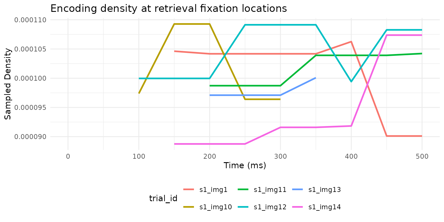
Encoding density sampled at retrieval fixation locations over time, for six example trials.
This reveals when during retrieval participants fixate locations that mattered during encoding — a window into the time course of memory-guided attention.
What’s next?
-
vignette("Multimatch")— compare scanpath structure across five dimensions -
vignette("RepetitiveSimilarity")— analyze repeated viewing of the same stimulus -
vignette("latent-transforms")— domain adaptation for cross-device or cross-participant comparisons - The package ships real data:
data(wynn_study)anddata(wynn_test)from a recognition memory experiment