Measuring Similarity Across Repeated Viewings
RepetitiveSimilarity.RmdWhen participants view the same image multiple times — say, during encoding and retrieval — do they look at the same locations each time? And is that consistency specific to the repeated stimulus, or just a general gaze pattern?
repetitive_similarity() answers these questions by
computing within-stimulus similarity across experimental conditions and
comparing it to cross-stimulus similarity. Unlike
template_similarity() which requires explicit
encoding-retrieval pairing, repetitive_similarity()
examines all possible within-stimulus combinations and
summarizes them.
Setting up the data
Let’s simulate a small dataset: 2 participants view 3 images during encoding and retrieval.
set.seed(42)

gen_fixations <- function(imname, phase, participant) {
  nfix <- sample(3:10, 1)
  data.frame(
    x = runif(nfix, 0, 100), y = runif(nfix, 0, 100),
    onset = cumsum(runif(nfix, 20, 80)),
    duration = runif(nfix, 80, 300),
    image = imname, phase = phase, participant = participant
  )
}

df <- do.call(rbind, lapply(c("s1", "s2"), function(s) {
  do.call(rbind, lapply(c("encoding", "retrieval"), function(p) {
    do.call(rbind, lapply(paste0("img", 1:3), function(img) {
      gen_fixations(img, p, s)
    }))
  }))
}))

eyetab <- eye_table("x", "y", "duration", "onset",
                    groupvar = c("participant", "phase", "image"),
                    data = df)
Compute density maps for each participant-phase-image combination:
eyedens <- density_by(eyetab,
                      groups = c("phase", "image", "participant"),
                      sigma = 50,
                      xbounds = c(0, 100), ybounds = c(0, 100))
Computing repetitive similarity
repetitive_similarity() takes the density table and a
condition variable (here phase) that defines the repeated
viewings:
rep_sim <- repetitive_similarity(eyedens,
                                 condition_var = "phase",
                                 method = "pearson")
rep_sim
#> # A tibble: 12 × 7
#>    phase     image participant fixgroup            density    repsim othersim
#>    <chr>     <chr> <chr>       <list>              <list>      <dbl>    <dbl>
#>  1 encoding  img1  s1          <fxtn_grp [3 × 6]>  <ey_dnsty> 0.304     0.367
#>  2 encoding  img1  s2          <fxtn_grp [9 × 6]>  <ey_dnsty> 0.377     0.626
#>  3 encoding  img2  s1          <fxtn_grp [6 × 6]>  <ey_dnsty> 0.423     0.506
#>  4 encoding  img2  s2          <fxtn_grp [6 × 6]>  <ey_dnsty> 0.461     0.694
#>  5 encoding  img3  s1          <fxtn_grp [10 × 6]> <ey_dnsty> 0.204     0.243
#>  6 encoding  img3  s2          <fxtn_grp [3 × 6]>  <ey_dnsty> 0.0566    0.388
#>  7 retrieval img1  s1          <fxtn_grp [9 × 6]>  <ey_dnsty> 0.688     0.582
#>  8 retrieval img1  s2          <fxtn_grp [5 × 6]>  <ey_dnsty> 0.531     0.408
#>  9 retrieval img2  s1          <fxtn_grp [5 × 6]>  <ey_dnsty> 0.534     0.565
#> 10 retrieval img2  s2          <fxtn_grp [3 × 6]>  <ey_dnsty> 0.341     0.389
#> 11 retrieval img3  s1          <fxtn_grp [7 × 6]>  <ey_dnsty> 0.538     0.587
#> 12 retrieval img3  s2          <fxtn_grp [5 × 6]>  <ey_dnsty> 0.312     0.293
The result contains two key columns:
- repsim — within-stimulus similarity: how consistently participants looked at the same locations for the same image across conditions
- othersim — cross-stimulus similarity: baseline similarity between different images viewed under different conditions
Interpreting the results
ggplot(rep_sim, aes(x = image, y = repsim)) +
  geom_col(fill = "steelblue", alpha = 0.7) +
  labs(x = "Stimulus", y = "Repetitive Similarity",
       title = "Same image across conditions") +
  theme_minimal()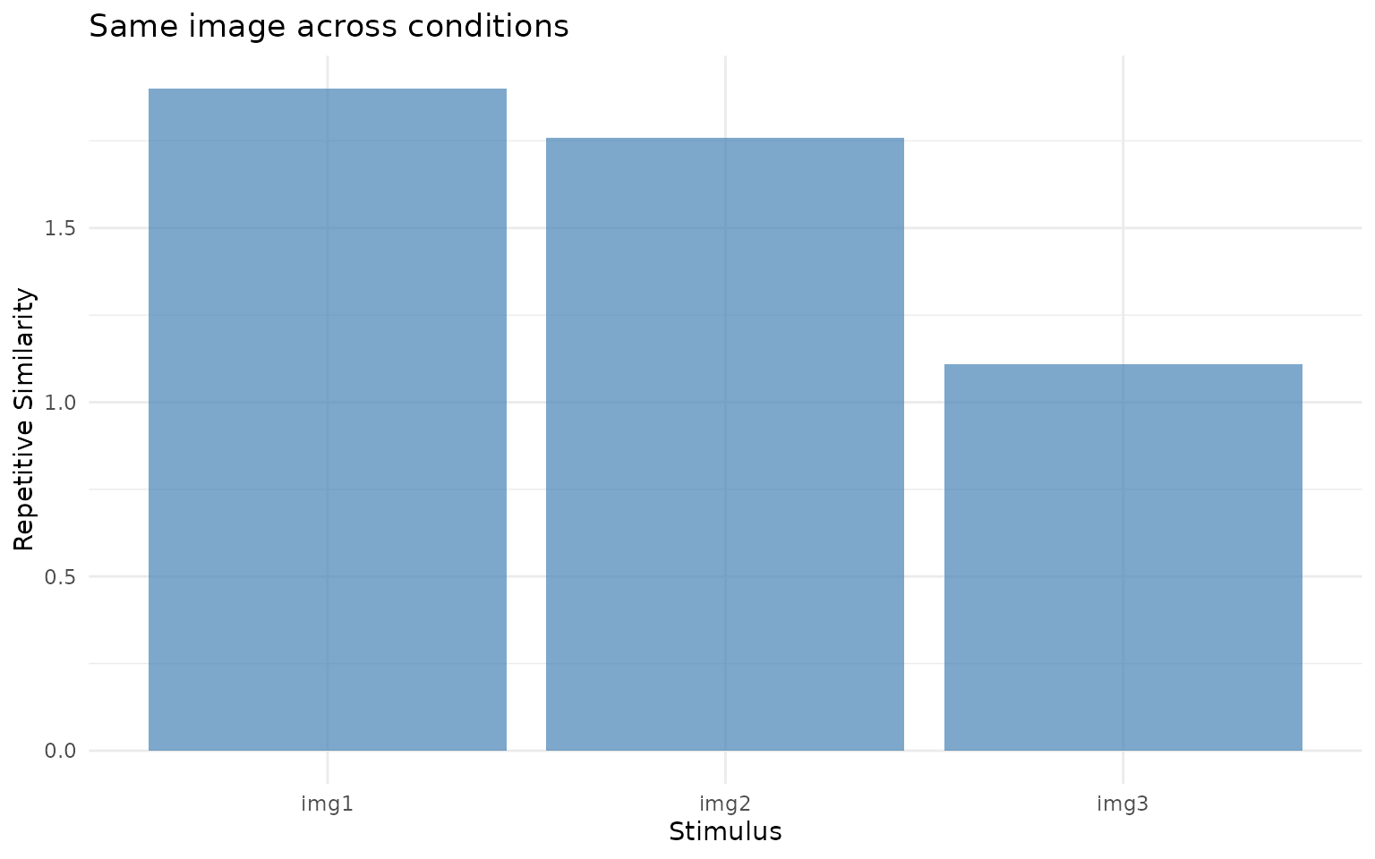
Within-stimulus similarity (repsim). Higher values indicate that participants fixated similar locations when viewing the same image across encoding and retrieval.
ggplot(rep_sim, aes(x = image, y = othersim)) +
  geom_col(fill = "coral", alpha = 0.7) +
  labs(x = "Stimulus", y = "Other Similarity",
       title = "Different images across conditions") +
  theme_minimal()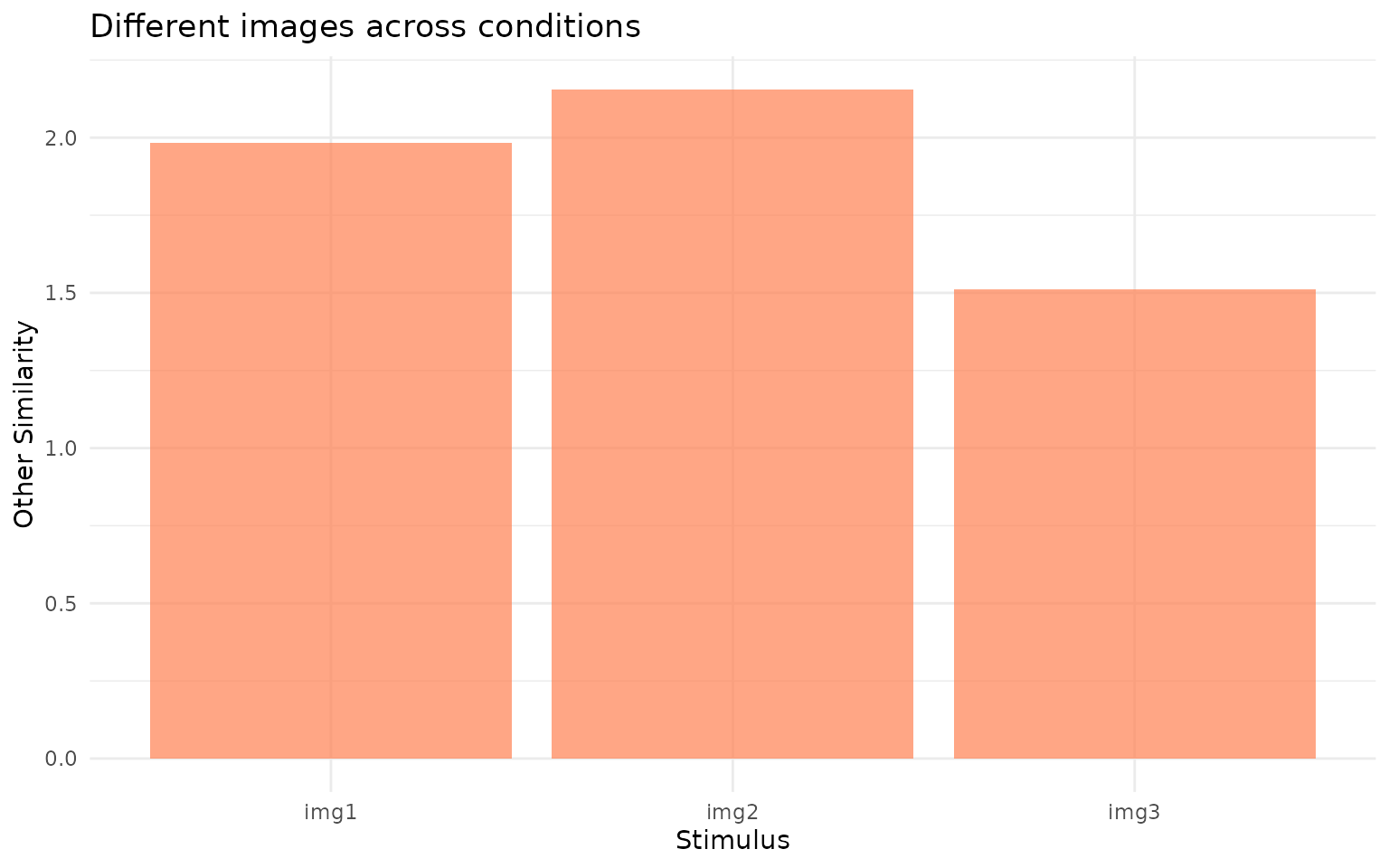
Cross-stimulus similarity (othersim). This represents the baseline: how similar gaze patterns are when comparing different images across conditions.
With random data, both values should be near zero. In a real
experiment, you would expect repsim to be higher than
othersim if participants show stimulus-specific
eye-movement reinstatement. The difference
(repsim - othersim) gives you a corrected measure of
reinstatement that controls for general gaze tendencies.
What’s next?
- See
?repetitive_similarityfor additional options, includingpairwise = TRUEto return all pairwise similarities instead of summaries -
vignette("eyesim")covers the fulltemplate_similarity()workflow with permutation-based baselines -
vignette("latent-transforms")describes domain-adaptation methods that can improve similarity estimates across devices or participants