PPC Analysis and Cluster Detection • bosc

The problem: finding rhythmic structure in noisy data

You’ve collected phase angles from neural recordings across many trials — perhaps from narrowband-filtered EEG time-locked to a behavioral response. Two questions arise:

Are the phases consistent across trials? If subjects respond at a preferred oscillatory phase, the phase distribution will be non-uniform.
Where in time-frequency space is the effect? With data at many frequencies and time points, you need cluster-based correction to control for multiple comparisons.

This vignette covers both: Pairwise Phase Consistency (PPC) for bias-free phase-locking measurement, and cluster-based permutation testing for time-frequency maps. PPC avoids the trial-count bias of mean resultant length, making it the preferred metric for comparing conditions with unequal trial numbers.

For oscillation score analysis, see vignette("oscillation-score").

Setup

library(bosc)

Pairwise Phase Consistency (PPC)

What is PPC?

PPC measures how consistent phase angles are across trials by computing the average cosine of pairwise phase differences:

$\text{PPC} = \frac{2}{n(n-1)} \sum_{i<j} \cos(\phi_i - \phi_j)$

PPC = 1: All phases identical (perfect consistency)
PPC = 0: Random phases (no consistency)
PPC < 0: Phases clustered at opposite angles

Basic PPC Computation

set.seed(123)

# Simulate phase data: 20 trials, 10 time points
n_trials <- 20

# Condition 1: Phases clustered around 0 (high consistency)
phases_consistent <- matrix(
  rnorm(n_trials * 10, mean = 0, sd = 0.3),
  nrow = n_trials
)

# Condition 2: Random phases (low consistency)
phases_random <- matrix(
  runif(n_trials * 10, -pi, pi),
  nrow = n_trials
)

# Compute PPC along trial dimension (dim = 1)
ppc_consistent <- pairwise_phase_consistency(phases_consistent, dim = 1)
ppc_random <- pairwise_phase_consistency(phases_random, dim = 1)
mean_ppc_consistent <- mean(ppc_consistent)
mean_ppc_random <- mean(ppc_random)

stopifnot(
  all(is.finite(ppc_consistent)),
  all(is.finite(ppc_random)),
  all(ppc_consistent <= 1),
  all(ppc_consistent >= -1),
  all(ppc_random <= 1),
  all(ppc_random >= -1),
  mean_ppc_consistent > mean_ppc_random
)

cat("PPC (consistent phases):", round(mean_ppc_consistent, 3), "\n")
#> PPC (consistent phases): 0.923
cat("PPC (random phases):", round(mean_ppc_random, 3), "\n")
#> PPC (random phases): -0.015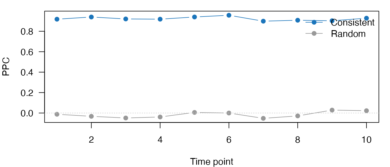

PPC values across time points: consistent phases (blue) vs random phases (grey).

Phase Extraction with Narrowband Hilbert

In real analyses, phases come from narrowband-filtered neural signals:

set.seed(456)
fs <- 500  # 500 Hz sampling

# Simulate 20 trials of oscillatory data with phase-locked response
n_trials <- 20
trial_length <- fs  # 1 second per trial

# Generate trials with consistent phase at response time
phases_at_response <- numeric(n_trials)
for (i in seq_len(n_trials)) {
  # Simulated neural signal: 10 Hz oscillation + noise
  t <- seq(0, 1, length.out = trial_length)
  neural <- sin(2 * pi * 10 * t + runif(1, -0.3, 0.3)) + rnorm(trial_length, sd = 0.5)

  # Extract alpha phase using narrowband Hilbert
  nb <- narrowband_hilbert(data = neural, fs = fs, freqlim = c(8, 12))

  # Get phase at "response time" (sample 250 = 500 ms)
  phases_at_response[i] <- Arg(nb$analytic[250])
}

# Compute circular statistics
cat("Mean phase:", round(circ_mean(phases_at_response), 3), "rad\n")
#> Mean phase: -1.608 rad
cat("Resultant length:", round(circ_r(phases_at_response), 3), "\n")
#> Resultant length: 0.984

# Rayleigh test
ray <- circ_rayleigh(phases_at_response)
stopifnot(
  all(is.finite(phases_at_response)),
  all(phases_at_response >= -pi),
  all(phases_at_response <= pi),
  is.finite(ray$pval),
  ray$pval >= 0,
  ray$pval <= 1
)

cat("Rayleigh p-value:", format(ray$pval, digits = 3), "\n")
#> Rayleigh p-value: 1.33e-08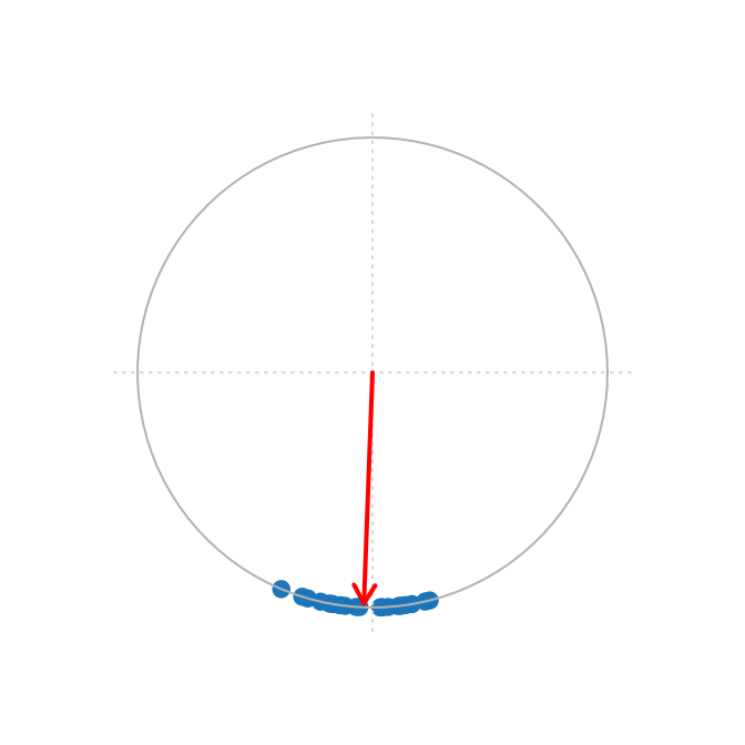

Phase angles at response time across 20 trials. Clustering near 0 indicates phase-locking.

Circular Statistics Functions

# Using the phases from consistent condition
angles <- phases_consistent[, 1]

# Circular mean direction
mu <- circ_mean(angles)
cat("Mean direction:", round(mu, 3), "rad\n")
#> Mean direction: 0.043 rad

# Mean resultant length (concentration)
r <- circ_r(angles)
cat("Resultant length:", round(r, 3), "\n")
#> Resultant length: 0.96

# Rayleigh test for non-uniformity
rayleigh <- circ_rayleigh(angles)
cat("Rayleigh p-value:", format(rayleigh$pval, digits = 3), "\n")
#> Rayleigh p-value: 2.44e-08

# V-test against expected direction of 0
vtest <- circ_vtest(angles, dir = 0)
stopifnot(
  is.finite(mu),
  is.finite(r),
  r >= 0,
  r <= 1,
  is.finite(rayleigh$pval),
  rayleigh$pval >= 0,
  rayleigh$pval <= 1,
  is.finite(vtest$pval),
  vtest$pval >= 0,
  vtest$pval <= 1
)

cat("V-test p-value:", format(vtest$pval, digits = 3), "\n")
#> V-test p-value: 6.48e-10

Visualizing Phase Distribution

plot_phase_hist(angles, nbins = 16)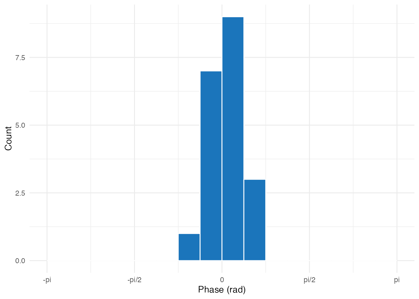

Phase distribution showing clustering around 0

How do you find significant clusters in time-frequency maps?

Cluster-based permutation testing is the standard approach for multiple comparison correction in time-frequency analyses. It works by:

Thresholding the statistical map to identify contiguous clusters
Computing a cluster statistic (sum of values)
Comparing against a null distribution from permutations

Simulating Time-Frequency Data

We start by creating two conditions for 15 subjects across a 30-frequency × 50-timepoint grid. The baseline condition is pure noise; we will add a localized effect in the second step.

set.seed(789)

n_freq <- 30
n_time <- 50
n_subjects <- 15

# Baseline condition: random noise across all subjects, frequencies, and times
baseline <- array(
  rnorm(n_subjects * n_freq * n_time, mean = 0, sd = 1),
  dim = c(n_subjects, n_freq, n_time)
)

# Effect condition starts identical in structure
effect <- array(
  rnorm(n_subjects * n_freq * n_time, mean = 0, sd = 1),
  dim = c(n_subjects, n_freq, n_time)
)

stopifnot(
  all(dim(baseline) == c(n_subjects, n_freq, n_time)),
  all(dim(effect) == c(n_subjects, n_freq, n_time)),
  all(is.finite(baseline)),
  all(is.finite(effect))
)

cat("Data dimensions:", dim(effect), "(subjects x freq x time)\n")
#> Data dimensions: 15 30 50 (subjects x freq x time)

Now we inject a spatially compact effect into the theta band (frequency rows 5–10) around the response window (time points 15–25). This mimics a real neural effect that cluster detection should recover.

# Add effect cluster (theta band: rows 5-10, time 15-25)
effect[, 5:10, 15:25] <- effect[, 5:10, 15:25] + 1.5
effect_mean <- mean(effect[, 5:10, 15:25])
baseline_mean <- mean(baseline[, 5:10, 15:25])

stopifnot(is.finite(effect_mean), is.finite(baseline_mean), effect_mean > baseline_mean)

cat("Effect magnitude added to rows 5:10, times 15:25\n")
#> Effect magnitude added to rows 5:10, times 15:25
cat("Mean in effect region (effect):", round(effect_mean, 3), "\n")
#> Mean in effect region (effect): 1.578
cat("Mean in effect region (baseline):", round(baseline_mean, 3), "\n")
#> Mean in effect region (baseline): 0.011

Computing T-scores

# Paired t-test across subjects (dimension 1)
tres <- paired_tscore(effect, baseline, dim = 1)
t_matrix <- matrix(tres$t, nrow = n_freq, ncol = n_time)
signal_window <- t_matrix[5:10, 15:25]

stopifnot(
  all(dim(t_matrix) == c(n_freq, n_time)),
  all(is.finite(t_matrix)),
  mean(signal_window) > 0
)

cat("T-score range:", round(range(t_matrix, na.rm = TRUE), 2), "\n")
#> T-score range: -3.94 9.06
cat("Max t-score location: freq", which.max(apply(t_matrix, 1, max)),
    ", time", which.max(apply(t_matrix, 2, max)), "\n")
#> Max t-score location: freq 9 , time 15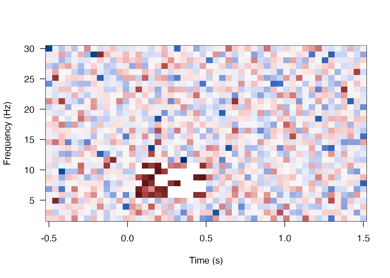

T-score map across frequency and time. The embedded effect cluster is visible in the theta range (rows 5-10, time 15-25).

Detecting Clusters

# Define frequency and time axes
freq_axis <- seq(2, 30, length.out = n_freq)
time_axis <- seq(-0.5, 1.5, length.out = n_time)

# Detect clusters using extract method
clusters <- detect_clusters(
  data = t_matrix,
  threshold = 2.0,  # t-threshold (roughly p < 0.05 uncorrected)
  method = "extract",
  smooth = 1,
  freq_axis = freq_axis,
  time_axis = time_axis
)

stopifnot(is.list(clusters))

cat("Number of clusters found:", length(clusters), "\n")
#> Number of clusters found: 1

# Examine clusters
if (length(clusters) > 0) {
  for (i in seq_along(clusters)) {
    cl <- clusters[[i]]
    stopifnot(
      length(cl$freqs) > 0,
      length(cl$times) > 0,
      all(is.finite(cl$freqs)),
      all(is.finite(cl$times)),
      is.finite(cl$sumZscore),
      is.finite(cl$peakZscore)
    )
    cat(sprintf("\nCluster %d:\n", i))
    cat(sprintf("  Frequency: %.1f - %.1f Hz\n", min(cl$freqs), max(cl$freqs)))
    cat(sprintf("  Time: %.2f - %.2f s\n", min(cl$times), max(cl$times)))
    cat(sprintf("  Size: %d pixels\n", length(cl$Zscores)))
    cat(sprintf("  Sum t: %.2f\n", cl$sumZscore))
    cat(sprintf("  Peak t: %.2f\n", cl$peakZscore))
  }
}
#> 
#> Cluster 1:
#>   Frequency: 5.9 - 10.7 Hz
#>   Time: 0.07 - 0.48 s
#>   Size: 65 pixels
#>   Sum t: 301.77
#>   Peak t: 9.06

Visualizing Clusters

plot_cluster_heatmap(
  data = t_matrix,
  clusters = clusters,
  freq_axis = freq_axis,
  time_axis = time_axis,
  zlim = c(-4, 4)
)

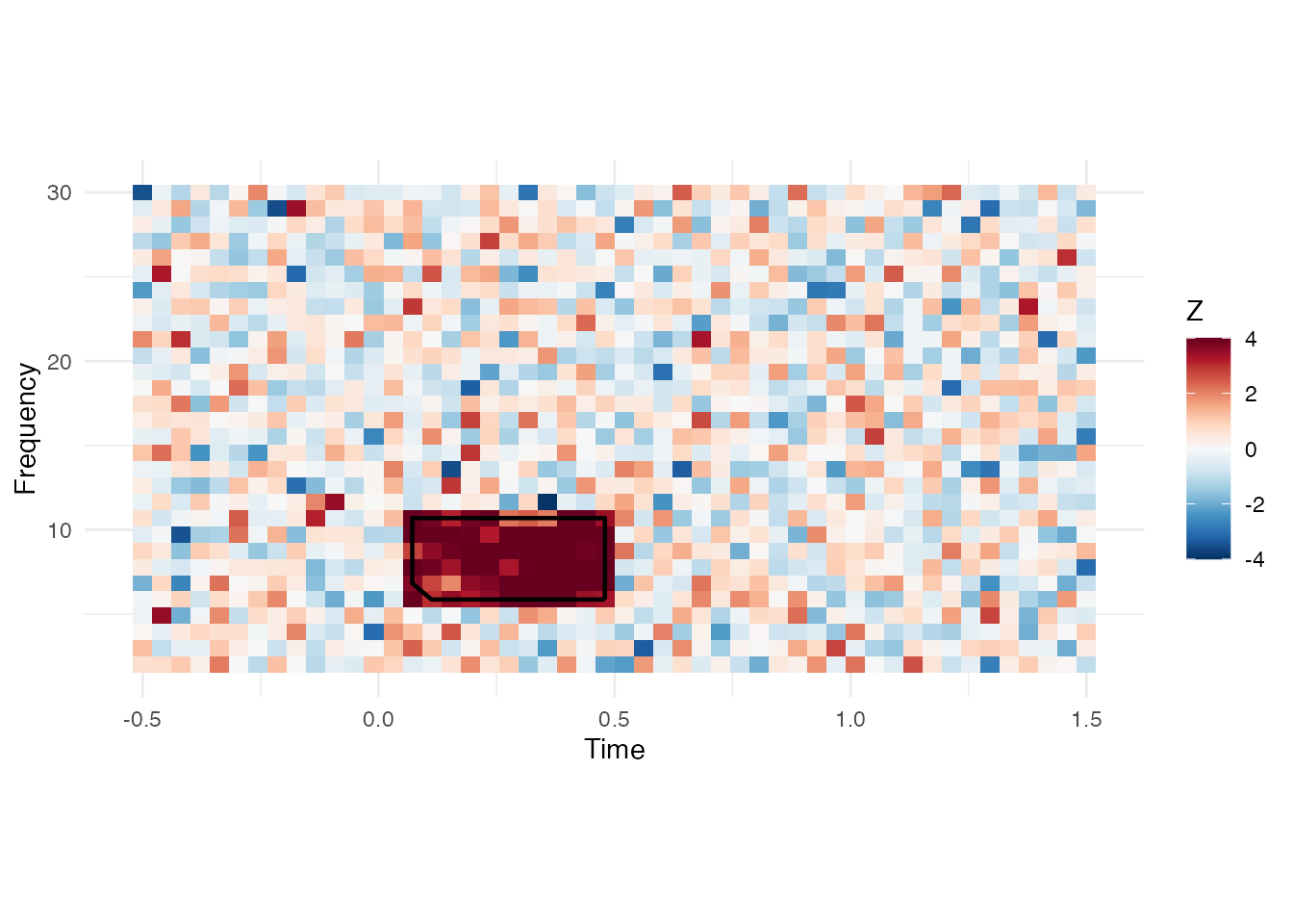
Time-frequency map with detected clusters outlined

Watershed vs Extract Methods

Two clustering methods are available:

Method	Description	Best for
`extract`	8-connectivity connected components	Sharply defined clusters
`watershed`	Watershed segmentation	Smooth, overlapping regions

# Watershed method (requires smoothing for best results)
clusters_ws <- detect_clusters(
  data = t_matrix,
  threshold = 2.0,
  method = "watershed",
  smooth = c(2, 2),  # smooth in both dimensions
  freq_axis = freq_axis,
  time_axis = time_axis
)

How do you correct for multiple comparisons?

FDR Correction

For element-wise testing without clustering, use FDR (False Discovery Rate):

# Convert t-scores to p-values
df <- n_subjects - 1
p_matrix <- 2 * pt(-abs(t_matrix), df = df)

# Apply Benjamini-Hochberg FDR correction
fdr_result <- fdr_bh(as.vector(p_matrix), q = 0.05)
stopifnot(
  all(is.finite(p_matrix)),
  all(p_matrix >= 0),
  all(p_matrix <= 1),
  length(fdr_result$h) == length(p_matrix),
  is.finite(fdr_result$crit_p),
  fdr_result$crit_p >= 0,
  fdr_result$crit_p <= 1
)

cat("Total tests:", length(p_matrix), "\n")
#> Total tests: 1500
cat("Significant after FDR:", sum(fdr_result$h), "\n")
#> Significant after FDR: 35
cat("Critical p-value:", format(fdr_result$crit_p, digits = 3), "\n")
#> Critical p-value: 0.000932

Non-parametric P-values

For permutation-based testing, use nonparam_pval():

set.seed(111)

# Observed statistics (can be a vector)
observed_stats <- c(15.5, 12.0, 8.5)

# Null distribution from permutations
null_distribution <- rnorm(1000, mean = 10, sd = 3)

# Compute p-values
result <- nonparam_pval(observed_stats, null_distribution)
stopifnot(
  length(result$p) == length(observed_stats),
  length(result$h) == length(observed_stats),
  all(is.finite(result$p)),
  all(result$p >= 0),
  all(result$p <= 1)
)

cat("Observed values:", observed_stats, "\n")
#> Observed values: 15.5 12 8.5
cat("P-values:", round(result$p, 4), "\n")
#> P-values: 0.03 0.252 0.299
cat("Significant (alpha=0.05):", result$h, "\n")
#> Significant (alpha=0.05): 1 0 0

U-Score Matrix (Non-parametric Testing)

For comparing observed values against a permutation distribution across a matrix:

set.seed(222)

# Observed values (2D matrix)
observed <- matrix(rnorm(20, mean = 0.5), nrow = 4, ncol = 5)

# Reference distribution (100 permutations)
reference <- array(rnorm(100 * 4 * 5), dim = c(100, 4, 5))

# Compute U-scores (position in null distribution)
u_result <- u_score_matrix(observed, reference, alpha = 0.05)
stopifnot(
  all(dim(u_result$Z) == dim(observed)),
  all(dim(u_result$sgnf) == dim(observed)),
  all(is.finite(u_result$Z))
)

cat("Significant elements:", sum(u_result$sgnf != 0), "of", length(observed), "\n")
#> Significant elements: 3 of 20

Putting it all together

Here’s a complete workflow combining PPC analysis with cluster detection:

set.seed(333)

# 1. Simulate PPC data: correct vs incorrect trials
n_subjects <- 12
n_freq <- 20
n_time <- 30

# Correct trials: higher theta PPC around response time
ppc_correct <- array(
  runif(n_subjects * n_freq * n_time, 0, 0.3),
  dim = c(n_subjects, n_freq, n_time)
)
# Add theta effect (freqs 3-6 = theta, times 10-20 = peri-response)
ppc_correct[, 3:6, 10:20] <- ppc_correct[, 3:6, 10:20] + 0.25

# Incorrect trials: baseline PPC
ppc_incorrect <- array(
  runif(n_subjects * n_freq * n_time, 0, 0.3),
  dim = c(n_subjects, n_freq, n_time)
)

# 2. Statistical comparison
diff_t <- paired_tscore(ppc_correct, ppc_incorrect, dim = 1)$t
diff_matrix <- matrix(diff_t, nrow = n_freq, ncol = n_time)
stopifnot(all(dim(diff_matrix) == c(n_freq, n_time)), all(is.finite(diff_matrix)))

# 3. Cluster detection
freq_ax <- seq(2, 30, length.out = n_freq)
time_ax <- seq(-0.2, 0.8, length.out = n_time)

sig_clusters <- detect_clusters(
  data = diff_matrix,
  threshold = 2.0,
  method = "extract",
  smooth = 1.5,
  freq_axis = freq_ax,
  time_axis = time_ax
)
stopifnot(is.list(sig_clusters))

# 4. Report
cat("=== PPC: Correct vs Incorrect Trials ===\n")
#> === PPC: Correct vs Incorrect Trials ===
cat("Subjects:", n_subjects, "\n")
#> Subjects: 12
cat("Clusters found:", length(sig_clusters), "\n\n")
#> Clusters found: 1

for (i in seq_along(sig_clusters)) {
  cl <- sig_clusters[[i]]
  cat(sprintf("Cluster %d:\n", i))
  cat(sprintf("  Frequency: %.1f - %.1f Hz\n", min(cl$freqs), max(cl$freqs)))
  cat(sprintf("  Time: %.2f - %.2f s\n", min(cl$times), max(cl$times)))
  cat(sprintf("  Center: %.1f Hz, %.2f s\n", cl$CoMfreq, cl$CoMtime))
  cat(sprintf("  Cluster t-sum: %.1f\n\n", cl$sumZscore))
}
#> Cluster 1:
#>   Frequency: 3.5 - 10.8 Hz
#>   Time: 0.08 - 0.49 s
#>   Center: 7.9 Hz, 0.28 s
#>   Cluster t-sum: 356.4

Working with real data

For actual experiments, use the I/O utilities:

# Load MATLAB .mat file (requires R.matlab package)
mat_data <- read_mat("path/to/ppc_data.mat")

# Access variables
ppc_matrix <- mat_data$ppc
freq_axis <- mat_data$freqs
time_axis <- mat_data$times

# Load HDF5 file (requires hdf5r package)
h5_file <- open_hdf5("path/to/data.h5")
ppc_matrix <- h5_file[["ppc"]][]
h5_file$close_all()

Next steps

Use oscillation_score_z() for one-call significance testing: vignette("workflow-wrappers")
Compute oscillation scores from spike trains: vignette("oscillation-score")
See ?pairwise_phase_consistency and ?detect_clusters for full argument lists

References

The algorithms in bosc are ported from the behavioral-oscillations MATLAB toolbox. Please cite:

Ter Wal, M. et al. (2021). Theta rhythmicity governs the timing of behavioural and hippocampal responses in humans specifically during memory-dependent tasks. Nature Communications, 12, 7048. https://doi.org/10.1038/s41467-021-27323-3