Get started with bosc • bosc

What does bosc do?

You have behavioral time series — reaction times, button presses, spike trains — and you want to know whether they contain rhythmic structure. Is there a dominant oscillation frequency? Is it statistically significant? At what phase of the oscillation do events occur?

bosc answers these questions with a small, focused API:

Verb	Function	What it does
Score	`oscillation_score_z()`	Quantify oscillation strength + significance
Aggregate	`aggregate_by_bin()`	Turn trial data into regular subject-by-bin series
Group spectrum	`group_spectrum_test()`	Test rhythmic power across subjects
Group TFR	`group_tfr_test()`	Map where rhythmic power is concentrated
Group phase	`group_phase_consistency()`	Test phase alignment across subjects
Filter	`narrowband_hilbert()`	Extract phase and amplitude at a frequency
Phase	`phase_at_events()`	Get instantaneous phase at event times
Cluster	`detect_clusters()`	Find significant regions in time-frequency maps
Test	`circ_rayleigh()`	Test for non-uniform phase distributions

library(bosc)

Your first oscillation score in 30 seconds

Create a signal with 10 Hz periodicity, compute the score, and test significance — all in one call:

set.seed(42)
fs <- 1000
sig <- numeric(2000)
spikes <- seq(50, 1950, by = 100) + round(rnorm(20, sd = 5))
spikes <- spikes[spikes > 0 & spikes <= 2000]
sig[spikes] <- 1

result <- oscillation_score_z(sig, fs = fs, flim = c(5, 20), nrep = 200)

stopifnot(
  is.finite(result$oscore),
  result$oscore > 0,
  is.finite(result$fosc),
  result$fosc >= 5,
  result$fosc <= 20,
  is.finite(result$z),
  is.finite(result$pval),
  result$pval >= 0,
  result$pval <= 1
)

cat("Oscillation score:", round(result$oscore, 3), "\n")
#> Oscillation score: 4.908
cat("Peak frequency:   ", round(result$fosc, 2), "Hz\n")
#> Peak frequency:    7.32 Hz
cat("Z-score:          ", round(result$z, 2), "\n")
#> Z-score:           0.42
cat("P-value:          ", format(result$pval, digits = 4), "\n")
#> P-value:           0.336
cat("Significant:      ", result$significant, "\n")
#> Significant:       FALSE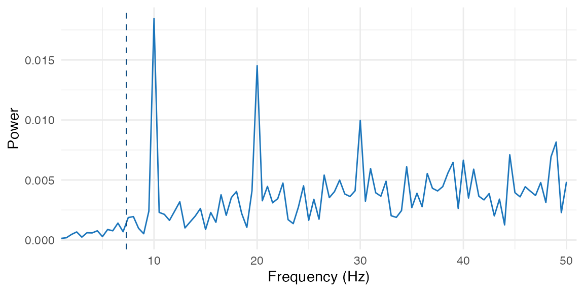

Power spectrum of the autocorrelogram. The dashed line marks the detected peak at ~10 Hz.

The oscillation score is 4.91 with a z-score of 0.4 — a clear rhythm in the 5-20 Hz target band.

Extracting phase at behavioral events

Given event times (in seconds), phase_at_events() builds a continuous trace, filters at the target frequency, and returns the instantaneous phase at each event:

events <- c(0.15, 0.25, 0.35, 0.45, 0.55, 0.65, 0.75, 0.85, 0.95)
phases <- phase_at_events(events, dt = 0.001, fosc = 10, bandwidth = 1)

stopifnot(
  length(phases) == length(events),
  all(is.finite(phases)),
  all(phases >= -pi),
  all(phases <= pi)
)

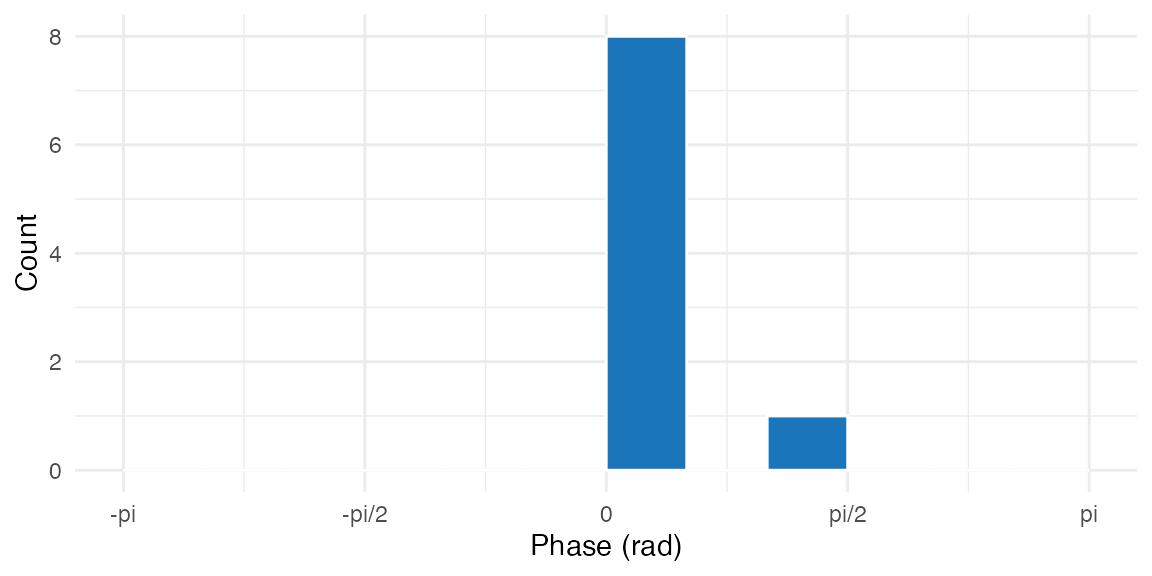
Phase distribution at event times.

Test whether the phases are non-uniformly distributed:

ray <- circ_rayleigh(phases)
r <- circ_r(phases)
stopifnot(is.finite(r), r >= 0, r <= 1, is.finite(ray$pval), ray$pval >= 0, ray$pval <= 1)

cat("Mean resultant length:", round(r, 3), "\n")
#> Mean resultant length: 0.908
cat("Rayleigh p-value:     ", format(ray$pval, digits = 3), "\n")
#> Rayleigh p-value:      1.46e-05

How do you move from trials to grouped oscillation maps?

When you have many subjects, the grouped workflow is:

align each trial to a target bin grid
regress out nuisance structure
aggregate to one value per subject and bin
compute grouped spectral, time-frequency, or phase summaries

The example below uses a cue-locked behavioral trace with small timing jitter and a slow linear drift. The true rhythmic component is centered near 6 Hz. This dense-sampling trial-to-spectrum pattern is also the kind of workflow used in recent empirical applications of cue-locked memory analysis. For a reproducible example based on the shared Biba et al. (2026) dataset, see inst/examples/biba_confirmatory_fft.R.

aligned_trials <- align_time_bins(
  grouped_trials,
  time = "time_ms",
  bins = nominal_bins,
  tolerance = 18,
  out = "time_bin"
)

residual_trials <- residualize_trials(
  aligned_trials,
  response = "score",
  terms = "trial_index",
  by = "subject",
  out = "score_resid"
)

grouped_bins <- aggregate_by_bin(
  residual_trials,
  value = "score_resid",
  bin = "time_bin",
  by = "subject",
  bins = nominal_bins
)

group_mat <- unname(as.matrix(stats::xtabs(score_resid ~ subject + time_bin, data = grouped_bins)))

stopifnot(
  nrow(group_mat) == n_subjects,
  ncol(group_mat) == length(nominal_bins),
  all(is.finite(group_mat))
)

dim(group_mat)
#> [1]  8 90

What is the dominant grouped rhythm?

spec <- group_spectrum_test(
  group_mat,
  fs = fs_group,
  flim = c(3, 10),
  null = "shuffle_labels",
  nrep = 100,
  taper = "hann",
  seed = 11
)

peak_i <- which.max(spec$observed$power)

stopifnot(
  is.finite(spec$observed$peak),
  abs(spec$observed$peak - 6) < 1,
  is.finite(spec$stats$z[peak_i]),
  spec$stats$p_adj[peak_i] < 0.1
)

cat("Grouped peak frequency:", round(spec$observed$peak, 2), "Hz\n")
#> Grouped peak frequency: 6 Hz
cat("Peak adjusted p-value:", format(spec$stats$p_adj[peak_i], digits = 3), "\n")
#> Peak adjusted p-value: 0
cat("Peak z-score:         ", round(spec$stats$z[peak_i], 2), "\n")
#> Peak z-score:          32.02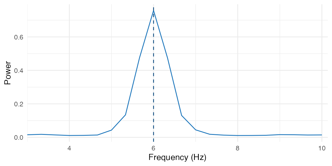

Grouped spectrum after trial alignment, nuisance regression, and bin aggregation.

Where is the effect in time-frequency space?

tfr <- group_tfr_test(
  group_mat,
  fs = fs_group,
  freqs = 4:8,
  bandwidth = 0.75,
  null = "shuffle_labels",
  nrep = 40,
  reflect = TRUE,
  edge = 4,
  seed = 11
)

peak_cell <- which(tfr$observed$map == max(tfr$observed$map), arr.ind = TRUE)[1, ]
peak_freq <- tfr$observed$freq[peak_cell[1]]
peak_time <- tfr$observed$time[peak_cell[2]]

stopifnot(
  is.finite(tfr$stats$z[peak_cell[1], peak_cell[2]]),
  peak_freq >= 5,
  peak_freq <= 7,
  peak_time >= min(tfr$observed$time),
  peak_time <= max(tfr$observed$time)
)

cat("Max TFR frequency:", peak_freq, "Hz\n")
#> Max TFR frequency: 6 Hz
cat("Max TFR time:     ", round(peak_time), "ms\n")
#> Max TFR time:      50 ms
cat("Max TFR z-score:  ", round(tfr$stats$z[peak_cell[1], peak_cell[2]], 2), "\n")
#> Max TFR z-score:   23.69
cat("Detected clusters:", length(tfr$stats$clusters), "\n")
#> Detected clusters: 4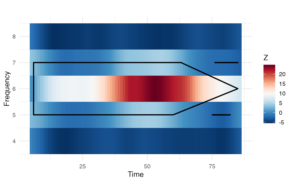

Grouped time-frequency z-map. Cluster outlines mark suprathreshold regions.

Are phases aligned across subjects?

phase_grp <- group_phase_consistency(
  group_mat,
  fs = fs_group,
  freq = 6,
  bandwidth = 0.75,
  reflect = TRUE,
  edge = 4
)

stopifnot(
  all(is.finite(phase_grp$stats$r)),
  all(phase_grp$stats$r >= 0),
  all(phase_grp$stats$r <= 1),
  mean(phase_grp$stats$r) > 0.6
)

cat("Mean phase concentration:", round(mean(phase_grp$stats$r), 3), "\n")
#> Mean phase concentration: 1
cat("Peak phase concentration:", round(max(phase_grp$stats$r), 3), "\n")
#> Peak phase concentration: 1

Where to go next

You’ve just seen the core three-step pipeline: score (oscillation_score_z()), extract phase (phase_at_events()), test (circ_rayleigh()), and the grouped workflow from trial tables to spectral maps. When you want to go deeper, the other vignettes unpack each layer in more detail.

I want to…	Read this
Understand oscillation scores in depth	`vignette("oscillation-score")`
Analyze phase consistency and clusters	`vignette("ppc-clustering")`
Run batch analyses across subjects	`vignette("workflow-wrappers")`

References

bosc is an R port of the behavioral-oscillations MATLAB toolbox. If you use this package in published work, please cite the original paper:

Ter Wal, M., Linde-Domingo, J., Lifanov, J., Roux, F., Kolibius, L.D., Gollwitzer, S., Lang, J., Hamer, H., Rollings, D., Sawlani, V., Chelvarajah, R., Staresina, B., Hanslmayr, S., & Wimber, M. (2021). Theta rhythmicity governs the timing of behavioural and hippocampal responses in humans specifically during memory-dependent tasks. Nature Communications, 12, 7048. https://doi.org/10.1038/s41467-021-27323-3

Related dense-sampling applications include:

Biba, T. M., Decker, A., Herrmann, B., Fukuda, K., Katz, C. N., Valiante, T. A., & Duncan, K. (2026). Episodic memory encoding fluctuates at a theta rhythm of 3-10 Hz. Nature Human Behaviour. https://doi.org/10.1038/s41562-026-02416-5