Running Batch Analyses and Extracting Phase • bosc

When you have many subjects and conditions

In a real experiment, you don’t analyze one signal — you analyze dozens of subjects across multiple conditions and frequency bands. Doing this with the low-level oscillation_score() and oscillation_score_surrogates() functions means writing the same boilerplate over and over: compute the score, run surrogates, calculate the z-score, test significance.

The workflow wrappers in bosc solve this by bundling common multi-step analyses into single calls. oscillation_score_z() gives you a score, surrogates, z-score, and p-value in one call. Config-list wrappers let you define parameters once and apply them across subjects. And phase_at_events() handles the full pipeline from event times to instantaneous phase.

library(bosc)

One call: score, surrogates, and significance

The most common workflow is computing an oscillation score and testing its significance against surrogates. oscillation_score_z() does this in one call:

# Generate a signal with 10 Hz periodicity
set.seed(42)
fs <- 1000
sig <- numeric(fs * 2)
spike_times <- seq(50, 1950, by = 100) + round(rnorm(20, sd = 5))
spike_times <- spike_times[spike_times > 0 & spike_times <= length(sig)]
sig[spike_times] <- 1

# One-call analysis: compute oscore, surrogates, and z-score
result <- oscillation_score_z(
  signal = sig,
  fs = fs,
  flim = c(5, 20),
  nrep = 200,
  alpha = 0.05,
  taper = "hanning"
)

stopifnot(
  is.finite(result$oscore),
  result$oscore > 0,
  is.finite(result$fosc),
  result$fosc >= 5,
  result$fosc <= 20,
  is.finite(result$z),
  is.finite(result$pval),
  result$pval >= 0,
  result$pval <= 1
)

cat("Oscillation score:", round(result$oscore, 3), "\n")
#> Oscillation score: 1.17
cat("Peak frequency:", round(result$fosc, 2), "Hz\n")
#> Peak frequency: 7.81 Hz
cat("Z-score:", round(result$z, 2), "\n")
#> Z-score: -1.47
cat("P-value:", format(result$pval, digits = 3), "\n")
#> P-value: 0.929
cat("Significant:", result$significant, "\n")
#> Significant: FALSE

How do you run the same analysis across subjects?

When running batch analyses across subjects or conditions, it’s convenient to define parameters once and reuse them. The _config wrappers accept named lists:

Define parameters once, apply everywhere

# Define analysis parameters
config <- list(
  fs = 1000,
  flim = c(1, 50),
  quantlim = c(0.05, 0.95),
  smoothach = TRUE,
  smoothwind = 0.002,
  peakwind = 0.008,
  taper = "hanning",
  warnings = "off"
)

# Apply to signal
os <- oscillation_score_config(config, sig)
stopifnot(
  is.finite(os$oscore),
  os$oscore > 0,
  is.finite(os$fosc),
  os$fosc >= config$flim[1],
  os$fosc <= config$flim[2]
)

cat("Oscillation score:", round(os$oscore, 3), "\n")
#> Oscillation score: 43.858
cat("Peak frequency:", round(os$fosc, 2), "Hz\n")
#> Peak frequency: 10.13 Hz

Adding surrogates to your config

# Extend config for surrogate analysis
config_sur <- modifyList(config, list(
  nrep = 200,
  fpeak = os$fosc,
  keep_trend = FALSE
))

sur <- oscillation_score_surrogates_config(config_sur, sig)

# Compute statistics from surrogate distribution
valid_sur <- sur$oscore_rp[is.finite(sur$oscore_rp) & sur$oscore_rp > 0]
z <- (log(os$oscore) - mean(log(valid_sur))) / sd(log(valid_sur))

stopifnot(
  length(valid_sur) >= 150,
  is.finite(z)
)

cat("Surrogate mean:", round(mean(sur$oscore_rp), 3), "\n")
#> Surrogate mean: 4.292
cat("Surrogate SD:", round(sd(sur$oscore_rp), 3), "\n")
#> Surrogate SD: 3.125
cat("Log-Z score:", round(z, 2), "\n")
#> Log-Z score: 3.13

Processing multiple subjects

# Simulate multiple subjects with varying oscillation strength
set.seed(123)
n_subjects <- 5

# Create subjects with different oscillation strengths
subjects <- lapply(1:n_subjects, function(i) {
  sig <- numeric(2000)
  # Vary jitter: stronger oscillation = less jitter
  jitter_sd <- 5 + (i - 1) * 3
  spikes <- seq(50, 1950, by = 100) + round(rnorm(20, sd = jitter_sd))
  spikes <- spikes[spikes > 0 & spikes <= 2000]
  sig[spikes] <- 1
  sig
})

# Apply same config to all subjects
results <- lapply(seq_along(subjects), function(i) {
  out <- oscillation_score_z(subjects[[i]], fs = 1000, flim = c(5, 20), nrep = 100)
  tidy_out <- oscore_tidy(out)
  tidy_out$subject <- i
  tidy_out[1, c("subject", "oscore", "fosc", "z", "significant")]
})

# Combine results
batch_results <- do.call(rbind, results)
stopifnot(
  nrow(batch_results) == n_subjects,
  all(c("subject", "oscore", "fosc", "z", "significant") %in% names(batch_results)),
  all(is.finite(batch_results$oscore)),
  all(is.finite(batch_results$fosc)),
  all(is.finite(batch_results$z))
)

print(batch_results[, c("subject", "oscore", "fosc", "z", "significant")])
#>   subject   oscore     fosc        z significant
#> 1       1 44.81143 9.765625 4.082184        TRUE
#> 2       2 48.91388 9.765625 4.250712        TRUE
#> 3       3 40.35858 9.765625 3.295853        TRUE
#> 4       4 26.09299 9.765625 2.609394        TRUE
#> 5       5 26.60936 9.765625 2.670983        TRUE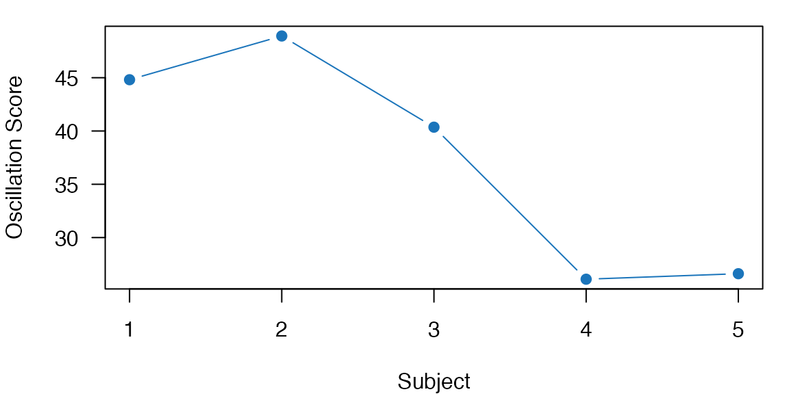

Oscillation scores across subjects with significant results highlighted in blue.

How do you extract phase at behavioral events?

A common analysis extracts the instantaneous phase of an oscillation at specific event times (e.g., button presses, stimulus onsets). phase_at_events() handles the full pipeline:

Convert event times to a continuous trace
Narrowband filter at the frequency of interest
Extract Hilbert phase at each event

# Event times in seconds (e.g., button presses)
events <- c(0.15, 0.25, 0.35, 0.45, 0.55, 0.65, 0.75, 0.85, 0.95)

# Extract phase at 10 Hz
phases <- phase_at_events(
  events = events,
  dt = 0.001,      # 1 ms time resolution
  fosc = 10,       # Center frequency
  bandwidth = 1    # +/- 1 Hz band
)
ray <- circ_rayleigh(phases)
stopifnot(
  length(phases) == length(events),
  all(is.finite(phases)),
  all(phases >= -pi),
  all(phases <= pi),
  is.finite(ray$pval),
  ray$pval >= 0,
  ray$pval <= 1
)

cat("Phases at events (radians):\n")
#> Phases at events (radians):
print(round(phases, 2))
#> [1] 0.06 0.07 0.06 0.06 0.05 0.05 0.07 0.18 1.52

# Check phase consistency
cat("\nMean resultant length:", round(circ_r(phases), 3), "\n")
#> 
#> Mean resultant length: 0.908
cat("Rayleigh p-value:", format(ray$pval, digits = 3), "\n")
#> Rayleigh p-value: 1.46e-05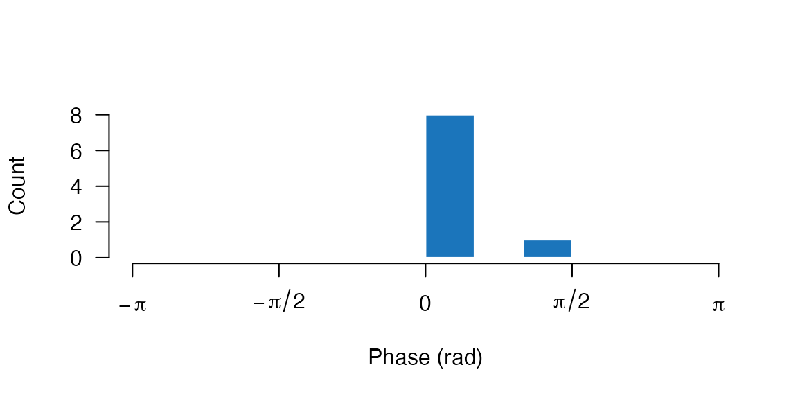

Phase distribution at event times. Clustering indicates phase-locked behavioral responses.

Leave-One-Out Phase Estimation

For unbiased phase estimation (avoiding circular analysis), use leave-one-out:

# Each event's phase is computed from a trace excluding that event
phases_loo <- phase_at_events(
  events = events,
  dt = 0.001,
  fosc = 10,
  bandwidth = 1,
  leave_one_out = TRUE
)

Getting results into data frames

The package includes helper functions to convert results to tidy data.frames, making it easy to combine results across analyses or use with ggplot2/dplyr. ### oscore_tidy: Oscillation Score Summaries

# Single result
os_tidy <- oscore_tidy(os)
stopifnot(all(c("oscore", "fosc") %in% names(os_tidy)))
os_tidy
#>     oscore     fosc     fmin     fmax
#> 1 43.85796 10.13184 1.681614 10.65022

# Can also handle oscillation_score_z output
z_result <- oscillation_score_z(sig, fs = 1000, flim = c(5, 20), nrep = 50)
z_tidy <- oscore_tidy(z_result)
stopifnot(all(c("oscore", "fosc", "z", "pval") %in% names(z_tidy)))
z_tidy
#>    oscore     fosc fmin     fmax         z      pval significant
#> 1 4.90813 7.324219    5 10.50972 0.3146127 0.3765279       FALSE

oscore_spectrum: Extract Spectrum Data

# Get spectrum as a data.frame for plotting
spec_df <- oscore_spectrum(os)
stopifnot(
  all(c("freq", "power") %in% names(spec_df)),
  all(is.finite(spec_df$freq)),
  all(is.finite(spec_df$power))
)

head(spec_df)
#>       freq        power
#> 1 1.708984 1.338058e-04
#> 2 1.831055 1.166433e-04
#> 3 1.953125 9.469540e-05
#> 4 2.075195 8.186402e-05
#> 5 2.197266 7.682177e-05
#> 6 2.319336 6.915301e-05

ggplot2::ggplot(spec_df, ggplot2::aes(x = freq, y = power)) +
  ggplot2::geom_line(color = "#1B75BB") +
  ggplot2::geom_vline(xintercept = os$fosc, linetype = "dashed", color = "red") +
  ggplot2::labs(x = "Frequency (Hz)", y = "Power") +
  ggplot2::theme_minimal()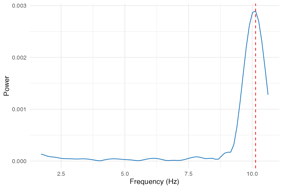

clusters_tidy: Cluster Summaries

After detecting clusters in time-frequency maps, convert to tidy format:

# Create example time-frequency data with clusters
set.seed(456)
n_freq <- 20
n_time <- 30
t_matrix <- matrix(rnorm(n_freq * n_time), nrow = n_freq)
# Add cluster
t_matrix[5:8, 10:15] <- t_matrix[5:8, 10:15] + 3

# Detect clusters
freq_axis <- seq(2, 30, length.out = n_freq)
time_axis <- seq(-0.2, 0.8, length.out = n_time)

clusters <- detect_clusters(
  data = t_matrix,
  threshold = 2.0,
  method = "extract",
  smooth = 1,
  freq_axis = freq_axis,
  time_axis = time_axis
)

# Convert to tidy summary
cluster_summary <- clusters_tidy(clusters)
stopifnot(all(c("cluster", "n_pixels", "freq_min", "time_min") %in% names(cluster_summary)))
print(cluster_summary[, c("cluster", "n_pixels", "freq_min", "freq_max",
                          "time_min", "time_max", "sumZscore")])
#>   cluster n_pixels freq_min freq_max  time_min  time_max sumZscore
#> 1       1       16 7.894737 12.31579 0.1103448 0.2827586  50.89751

clusters_pixels: Per-Pixel Data

For detailed analysis or custom plotting, get all cluster pixels:

# Get all pixels from detected clusters
pixel_df <- clusters_pixels(clusters)
stopifnot(
  nrow(pixel_df) > 0,
  all(c("time", "freq", "Zscore") %in% names(pixel_df)),
  all(is.finite(pixel_df$time)),
  all(is.finite(pixel_df$freq)),
  all(is.finite(pixel_df$Zscore))
)

head(pixel_df)
#>   cluster      time      freq   Zscore pAdj
#> 1       1 0.1103448  9.368421 2.899204   NA
#> 2       1 0.1103448 10.842105 4.070153   NA
#> 3       1 0.1448276  9.368421 1.927576   NA
#> 4       1 0.1448276 10.842105 2.432312   NA
#> 5       1 0.1448276 12.315789 3.129383   NA
#> 6       1 0.1793103  9.368421 3.600278   NA

ggplot2::ggplot(pixel_df, ggplot2::aes(x = time, y = freq, fill = Zscore)) +
  ggplot2::geom_tile() +
  ggplot2::scale_fill_gradient2(low = "blue", mid = "white", high = "red", midpoint = 0) +
  ggplot2::labs(x = "Time (s)", y = "Frequency (Hz)", fill = "Z-score") +
  ggplot2::theme_minimal()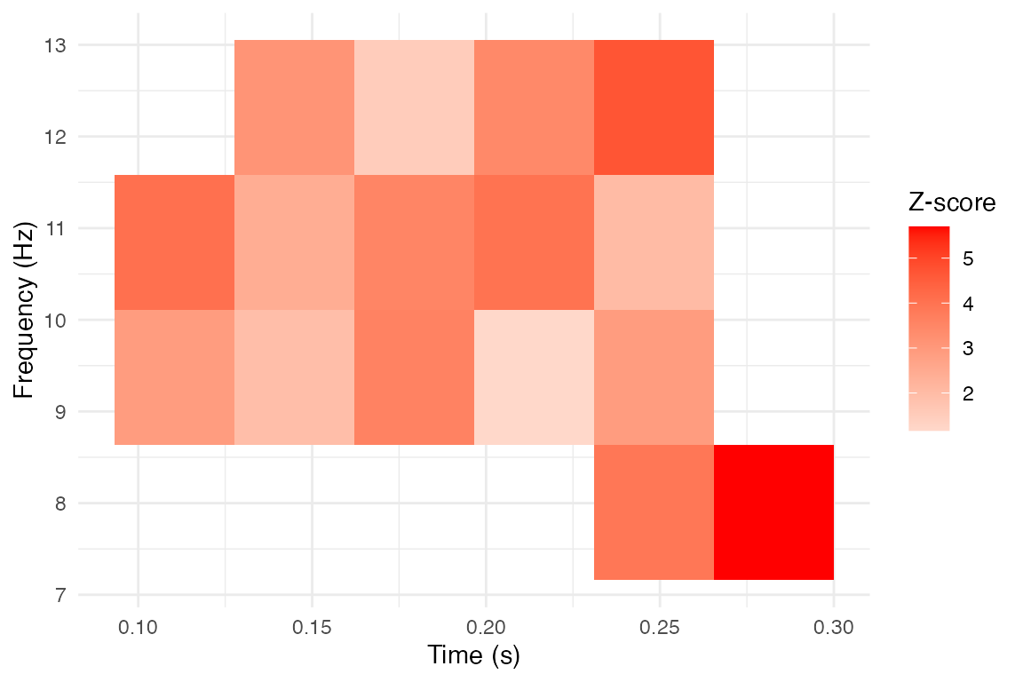

Putting it all together

Here’s a complete example combining the workflow wrappers:

set.seed(789)

# 1. Generate behavioral data with oscillatory structure
fs <- 1000
duration <- 3
n_samples <- fs * duration

# Response times with 8 Hz periodicity
base_times <- seq(0.1, 2.9, by = 0.125)  # 8 Hz
event_times <- base_times + rnorm(length(base_times), sd = 0.01)
event_times <- sort(event_times[event_times > 0 & event_times < duration])

# Convert to spike train
sig <- numeric(n_samples)
sig[round(event_times * fs)] <- 1

# 2. Compute oscillation score with significance
config <- list(
  fs = fs,
  flim = c(4, 15),
  nrep = 200,
  alpha = 0.05,
  taper = "hanning"
)

z_result <- oscillation_score_z(
  signal = sig,
  fs = config$fs,
  flim = config$flim,
  nrep = config$nrep,
  alpha = config$alpha,
  taper = config$taper
)
stopifnot(
  is.finite(z_result$oscore),
  z_result$oscore > 0,
  is.finite(z_result$fosc),
  z_result$fosc >= config$flim[1],
  z_result$fosc <= config$flim[2],
  is.finite(z_result$z),
  is.finite(z_result$pval),
  z_result$pval >= 0,
  z_result$pval <= 1
)

# 3. Extract phases at response times
phases <- phase_at_events(
  events = event_times,
  dt = 1/fs,
  fosc = z_result$fosc,
  bandwidth = 1
)
stopifnot(
  length(phases) == length(event_times),
  all(is.finite(phases)),
  all(phases >= -pi),
  all(phases <= pi)
)

# 4. Test phase consistency
ray <- circ_rayleigh(phases)
stopifnot(is.finite(ray$pval), ray$pval >= 0, ray$pval <= 1)

# 5. Report results
cat("=== Oscillation Analysis Results ===\n\n")
#> === Oscillation Analysis Results ===

cat("Oscillation Score Analysis:\n")
#> Oscillation Score Analysis:
cat(sprintf("  O-score: %.3f\n", z_result$oscore))
#>   O-score: 50.978
cat(sprintf("  Peak frequency: %.2f Hz\n", z_result$fosc))
#>   Peak frequency: 7.81 Hz
cat(sprintf("  Z-score: %.2f\n", z_result$z))
#>   Z-score: 3.44
cat(sprintf("  P-value: %.4f\n", z_result$pval))
#>   P-value: 0.0003
cat(sprintf("  Significant: %s\n\n", z_result$significant))
#>   Significant: TRUE

cat("Phase Consistency:\n")
#> Phase Consistency:
cat(sprintf("  Mean phase: %.2f rad\n", circ_mean(phases)))
#>   Mean phase: 0.12 rad
cat(sprintf("  Resultant length: %.3f\n", circ_r(phases)))
#>   Resultant length: 0.906
cat(sprintf("  Rayleigh p-value: %.4f\n", ray$pval))
#>   Rayleigh p-value: 0.0000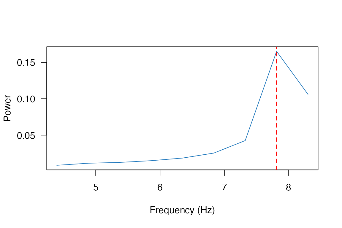

Power spectrum from the complete pipeline. The dashed line marks the detected peak frequency.

Next steps

Compute oscillation scores from scratch: vignette("oscillation-score")
Analyze phase consistency and clusters: vignette("ppc-clustering")
See ?oscillation_score_z and ?phase_at_events for full argument lists

References

The algorithms in bosc are ported from the behavioral-oscillations MATLAB toolbox. Please cite:

Ter Wal, M. et al. (2021). Theta rhythmicity governs the timing of behavioural and hippocampal responses in humans specifically during memory-dependent tasks. Nature Communications, 12, 7048. https://doi.org/10.1038/s41467-021-27323-3