Quick start: plot()
The simplest way to visualize a volume is the S4 plot()
method. It shows a 3 x 3 montage of evenly-spaced axial slices with a
perceptually uniform grayscale palette and clean theme.
plot(vol)                       # 3x3 montage, grayscale
plot(vol, cmap = "viridis")     # different palette
plot(vol, overlay)              # overlay with inferno palette, alpha = 0.5
plot(vol, overlay, ov_alpha = 0.7, ov_thresh = 2)
For more control — coronal/sagittal planes, downsampling, custom facet layouts — the dedicated helpers below give full flexibility.
Why these helpers?
Neuroimaging images are large, orientation-sensitive rasters. The goal of these helpers is to make reasonable defaults easy to use: perceptually uniform palettes, robust scaling, fixed aspect ratios, and clean legends — without extra heavy dependencies or any JavaScript.
This vignette shows how to:
- Build publication-ready montages
- Create a compact orthogonal (three-plane) view with crosshairs
- Overlay a statistical map on a structural background (threshold + alpha)
The helpers used here are:
-
resolve_cmap(),scale_fill_neuro(),theme_neuro() -
plot_montage(),plot_ortho(),plot_overlay() annotate_orientation()
Getting a demo volume
The examples below try to read a sample NIfTI included with the
package. If that is not available, they create a small synthetic 3D
volume and wrap it in NeuroVol. Either way, the rest of the
code is identical.
set.seed(1)

make_synthetic_vol <- function(dims = c(96, 96, 72), vox = c(2, 2, 2)) {
  i <- array(rep(seq_len(dims[1]), times = dims[2]*dims[3]), dims)
  j <- array(rep(rep(seq_len(dims[2]), each = dims[1]), times = dims[3]), dims)
  k <- array(rep(seq_len(dims[3]), each = dims[1]*dims[2]), dims)

  c0 <- dims / 2
  g1 <- exp(-((i - c0[1])^2 + (j - c0[2])^2 + (k - c0[3])^2) / (2*(min(dims)/4)^2))
  g2 <- 0.5 * exp(-((i - (c0[1] + 15))^2 + (j - (c0[2] - 10))^2 + (k - (c0[3] + 8))^2) / (2*(min(dims)/6)^2))
  x  <- g1 + g2 + 0.05 * array(stats::rnorm(prod(dims)), dims)

  sp <- NeuroSpace(dims, spacing = vox)
  NeuroVol(x, sp)
}

# Prefer an included demo file. Use a real example from inst/extdata.
demo_path <- system.file("extdata", "mni_downsampled.nii.gz", package = "neuroim2")

t1 <- if (nzchar(demo_path)) {
  read_vol(demo_path)
} else {
  make_synthetic_vol()
}

dims <- dim(t1)

# Build a synthetic "z-statistic" overlay matched to t1's dims
mk_blob <- function(mu, sigma = 8) {
  i <- array(rep(seq_len(dims[1]), times = dims[2]*dims[3]), dims)
  j <- array(rep(rep(seq_len(dims[2]), each = dims[1]), times = dims[3]), dims)
  k <- array(rep(seq_len(dims[3]), each = dims[1]*dims[2]), dims)
  exp(-((i - mu[1])^2 + (j - mu[2])^2 + (k - mu[3])^2) / (2*sigma^2))
}
ov_arr <- 3.5 * mk_blob(mu = round(dims * c(.60, .45, .55)), sigma = 7) -
          3.2 * mk_blob(mu = round(dims * c(.35, .72, .40)), sigma = 6) +
          0.3 * array(stats::rnorm(prod(dims)), dims)

overlay <- NeuroVol(ov_arr, space(t1))
1) Montages that read well at a glance
The montage helper facets a single ggplot object—so you get a shared colorbar, clean panel labels, and proper aspect ratio.
# Choose a sensible set of axial slices
zlevels <- unique(round(seq( round(dims[3]*.25), round(dims[3]*.85), length.out = 12 )))

p <- plot_montage(
  t1, zlevels = zlevels, along = 3,
  cmap = "grays", range = "robust", probs = c(.02, .98),
  ncol = 6, title = "Axial montage (robust scaling)"
)
p + theme_neuro()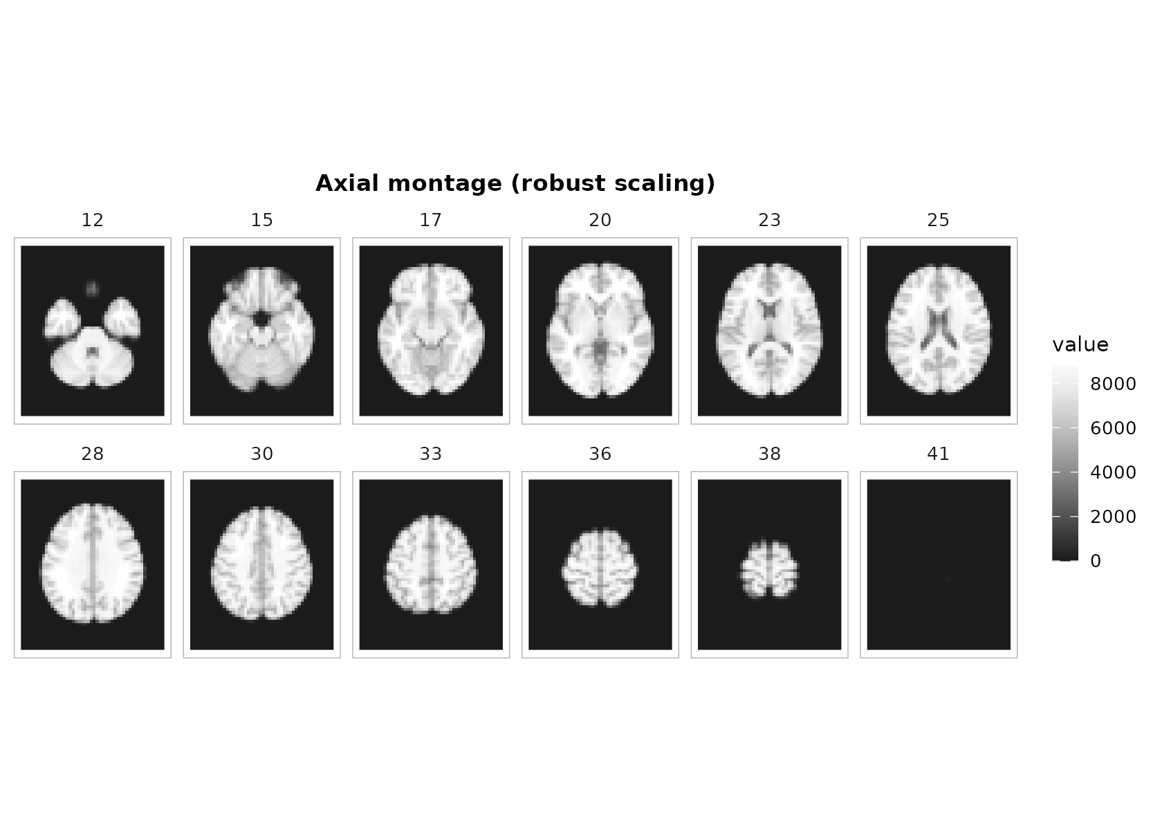
Notes
-
range = "robust"uses quantiles (default 2–98%) to ignore outliers. -
coord_fixed()+ reversed y are handled internally to preserve geometry and radiological convention. - Use
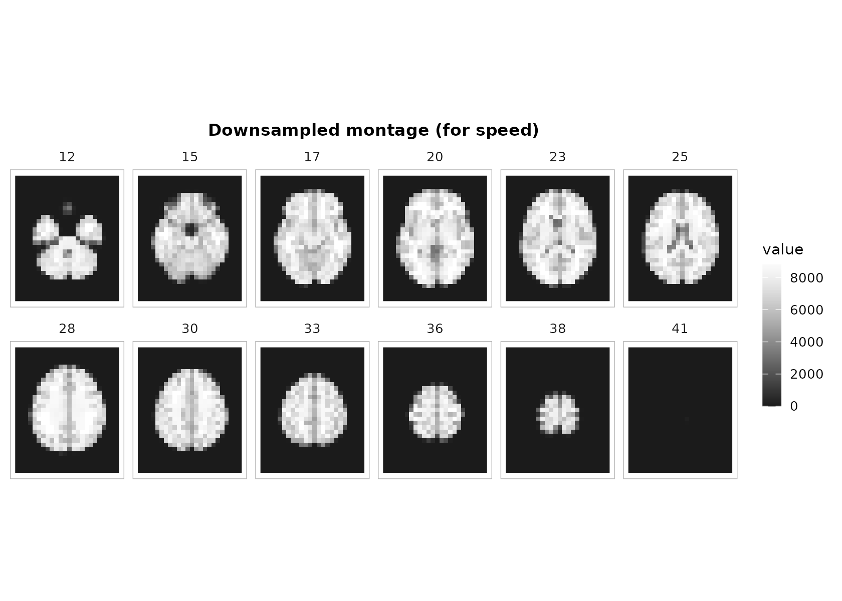
downsample = 2(or higher) when plotting huge volumes interactively.
plot_montage(
  t1, zlevels = zlevels, along = 3,
  cmap = "grays", range = "robust", ncol = 6, downsample = 2,
  title = "Downsampled montage (for speed)"
)
2) Orthogonal three‑plane view (with crosshairs)
plot_ortho() produces aligned sagittal, coronal, and
axial slices with a shared scale, optional crosshairs, and compact
orientation glyphs.
center_voxel <- round(dim(t1) / 2)
plot_ortho(
  t1, coord = center_voxel, unit = "index",
  cmap = "grays", range = "robust",
  crosshair = TRUE, annotate = TRUE
)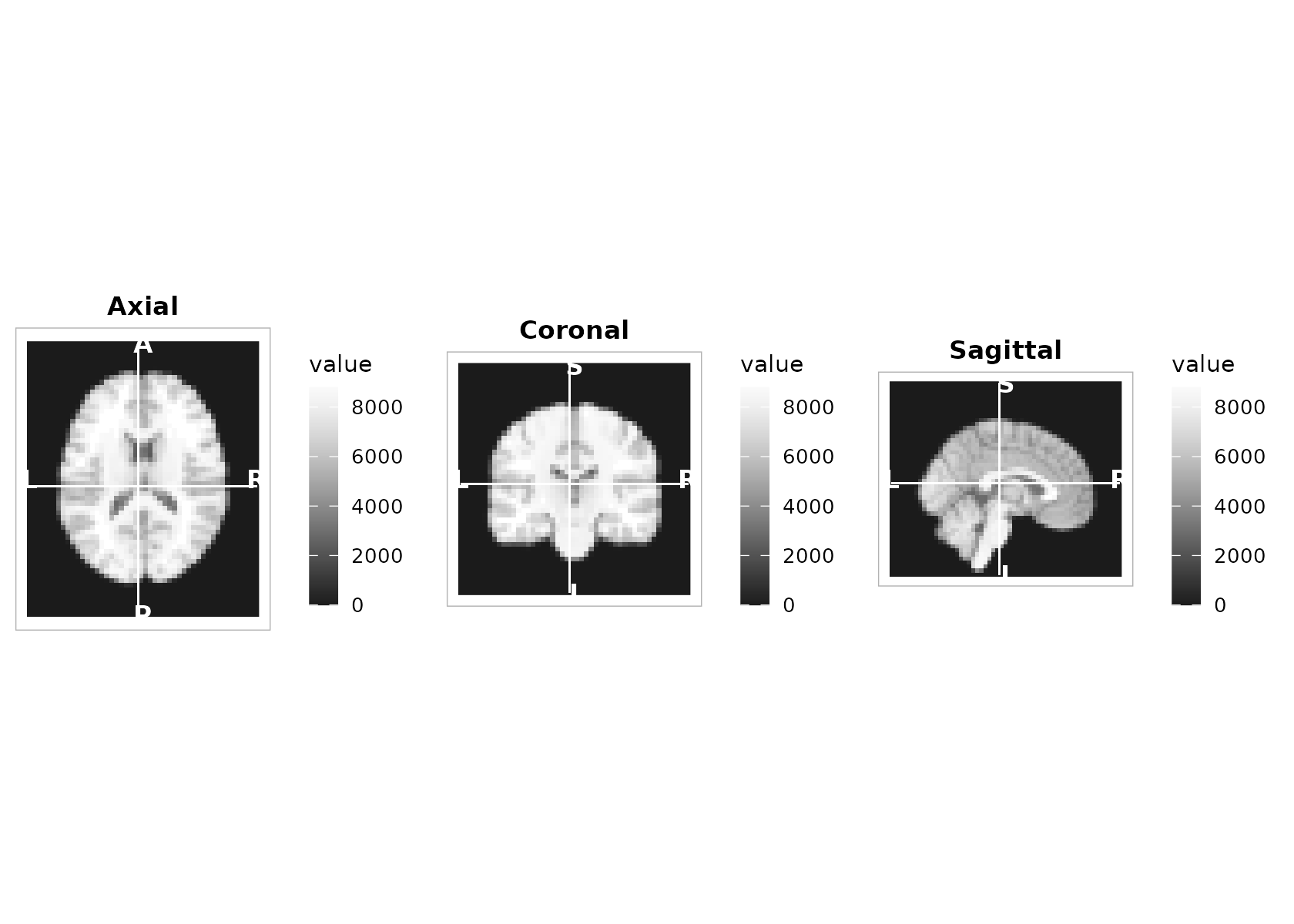
Tip: If you have MNI/world coordinates, pass unit = "mm"
and a length‑3 numeric; internally it will convert using
coord_to_grid(space(vol), …) if available.
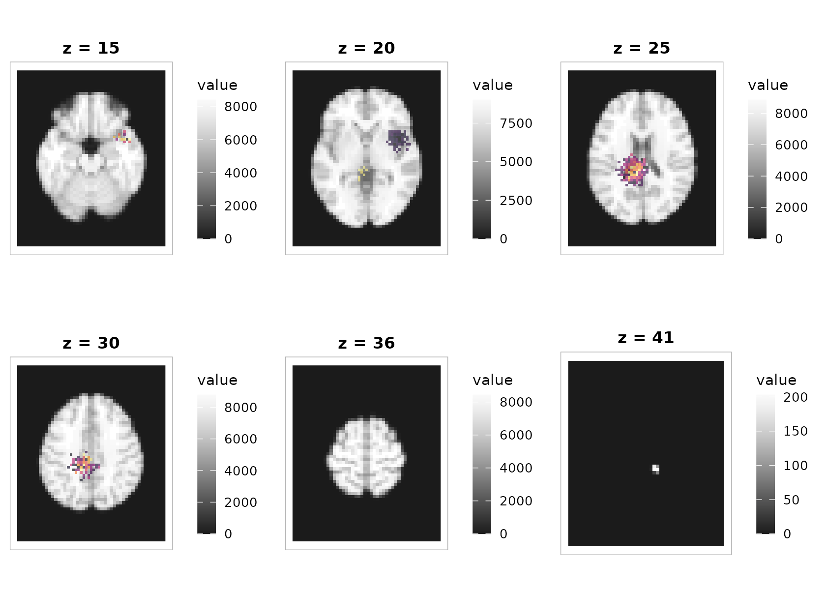
3) Overlaying an activation map on a structural background
The overlay compositor colorizes each layer independently (so each can use its own limits and palette) and stacks them as rasters. No extra packages required.
plot_overlay(
  bgvol = t1, overlay = overlay,
  zlevels = zlevels[seq(2, length(zlevels), by = 2)],  # fewer panels for the vignette
  bg_cmap = "grays", ov_cmap = "inferno",
  bg_range = "robust", ov_range = "robust", probs = c(.02, .98),
  ov_thresh = 2.5,   # make weaker signal transparent
  ov_alpha  = 0.65,
  ncol = 3, title = "Statistical overlay (threshold 2.5, alpha 0.65)"
)
4) Palettes and aesthetics
All examples above use neuro‑friendly defaults:
- Palettes:
resolve_cmap()wraps base R’shcl.colors()with aliases like “grays”, “viridis”, “inferno”—and safe fallbacks. - Theme:
theme_neuro()keeps panels quiet and legends slim. - Legend: one shared colorbar for facetted montages via
scale_fill_neuro().
You can switch palettes easily:
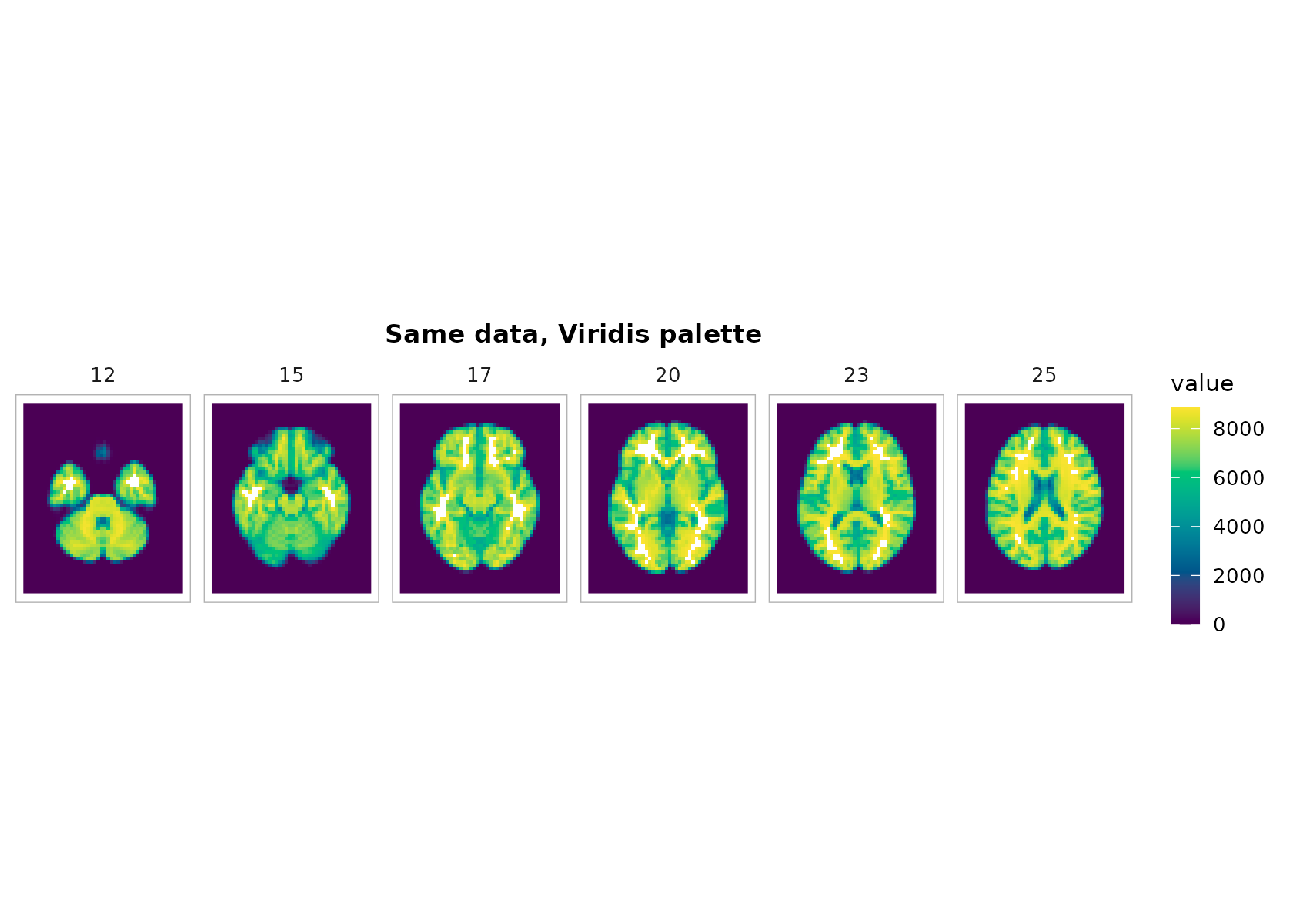
plot_montage(
  t1, zlevels = zlevels[1:6], along = 3,
  cmap = "viridis", range = "robust", ncol = 6,
  title = "Same data, Viridis palette"
)
5) Practical tips
- Choose slices with meaning. Use mm positions (if you have an affine) or meaningful indices; label strips are handled for you by the helper.
- Speed vs. fidelity. Use
downsamplefor exploration; keepdownsample = 1for final figures. - Consistent limits. For side‑by‑side comparisons, compute limits on a combined set of values (the helpers do this for orthogonal panels automatically).
Reproducibility
sessionInfo()
## R version 4.6.0 (2026-04-24)
## Platform: x86_64-pc-linux-gnu
## Running under: Ubuntu 24.04.4 LTS
##
## Matrix products: default
## BLAS:   /usr/lib/x86_64-linux-gnu/openblas-pthread/libblas.so.3
## LAPACK: /usr/lib/x86_64-linux-gnu/openblas-pthread/libopenblasp-r0.3.26.so;  LAPACK version 3.12.0
##
## locale:
##  [1] LC_CTYPE=C.UTF-8       LC_NUMERIC=C           LC_TIME=C.UTF-8
##  [4] LC_COLLATE=C.UTF-8     LC_MONETARY=C.UTF-8    LC_MESSAGES=C.UTF-8
##  [7] LC_PAPER=C.UTF-8       LC_NAME=C              LC_ADDRESS=C
## [10] LC_TELEPHONE=C         LC_MEASUREMENT=C.UTF-8 LC_IDENTIFICATION=C
##
## time zone: UTC
## tzcode source: system (glibc)
##
## attached base packages:
## [1] stats     graphics  grDevices utils     datasets  methods   base
##
## other attached packages:
## [1] neuroim2_0.16.0 Matrix_1.7-5    ggplot2_4.0.3
##
## loaded via a namespace (and not attached):
##  [1] sass_0.4.10           generics_0.1.4        mmap_0.6-26
##  [4] stringi_1.8.7         lattice_0.22-9        digest_0.6.39
##  [7] magrittr_2.0.5        bigstatsr_1.6.2       evaluate_1.0.5
## [10] grid_4.6.0            RColorBrewer_1.1-3    iterators_1.0.14
## [13] rmio_0.4.0            fastmap_1.2.0         foreach_1.5.2
## [16] doParallel_1.0.17     jsonlite_2.0.0        RNifti_1.9.0
## [19] purrr_1.2.2           deflist_0.2.0         scales_1.4.0
## [22] albersdown_1.0.1      codetools_0.2-20      textshaping_1.0.5
## [25] jquerylib_0.1.4       cli_3.6.6             rlang_1.2.0
## [28] cowplot_1.2.0         splines_4.6.0         withr_3.0.2
## [31] cachem_1.1.0          yaml_2.3.12           flock_0.7
## [34] tools_4.6.0           parallel_4.6.0        memoise_2.0.1
## [37] bigassertr_0.1.7      assertthat_0.2.1      vctrs_0.7.3
## [40] R6_2.6.1              lifecycle_1.0.5       bigparallelr_0.3.2
## [43] stringr_1.6.0         fs_2.1.0              dbscan_1.2.4
## [46] ragg_1.5.2            pkgconfig_2.0.3       desc_1.4.3
## [49] pkgdown_2.2.0         RcppParallel_5.1.11-2 bslib_0.10.0
## [52] pillar_1.11.1         gtable_0.3.6          glue_1.8.1
## [55] Rcpp_1.1.1-1.1        systemfonts_1.3.2     xfun_0.57
## [58] tibble_3.3.1          knitr_1.51            farver_2.1.2
## [61] htmltools_0.5.9       labeling_0.4.3        RNiftyReg_2.8.5
## [64] rmarkdown_2.31        compiler_4.6.0        S7_0.2.2