Wang Visual Cortex Atlas: Surface and Volume • neuroatlas

The Wang et al. (2015) atlas describes 25 retinotopic and functional visual areas per hemisphere. neuroatlas exposes two related products: a labelled fsaverage surface atlas and the authors’ probabilistic volume distribution. They share a region vocabulary, but they are not interchangeable coordinate representations.

Network-backed chunks are displayed but not executed during package builds. The figures are committed outputs generated from the code shown.

Which product should you use?

Scientific question	Loader	Representation
where do areas lie on cortex?	`get_wang_atlas()`	`surfatlas` in `fsaverage` / MNI305 coordinates
what is the maximum-probability voxel label?	`get_wang_prob_atlas(image = "maxprob")`	raw `NeuroVol` pair on the native ProbAtlas grid
what probability does one area have at each voxel?	`get_wang_prob_atlas(image = "probability")`	raw continuous `NeuroVol` objects

Choose the representation from the analysis, not from which picture is easier to make.

How do you load the native surface atlas?

get_wang_atlas() returns 50 regions: the same 25 area names in each hemisphere. The default midthickness geometry and label overlays may be downloaded and cached on first use.

library(neuroatlas)

wang <- get_wang_atlas(surf = "midthickness")
meta <- roi_metadata(wang)

stopifnot(
  inherits(wang, "surfatlas"),
  length(wang$ids) == 50L,
  all(table(wang$hemi) == c(left = 25L, right = 25L)),
  atlas_ref(wang)$template_space == "fsaverage",
  atlas_ref(wang)$coord_space == "MNI305"
)

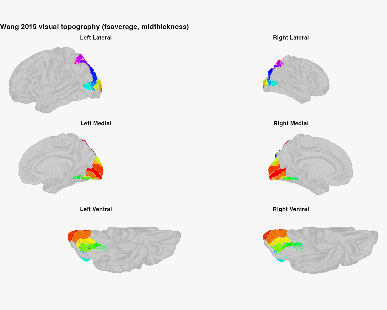
The medial and ventral views reveal early and ventral visual cortex; lateral views show dorsal and lateral areas. background = TRUE keeps the unlabelled cortex visible as anatomical context.

plot_brain(
  wang,
  views = c("lateral", "medial", "ventral"),
  interactive = FALSE,
  style = "ggseg_like",
  background = TRUE,
  title = "Wang 2015 visual topography (fsaverage, midthickness)"
)

Wang visual areas shown on lateral, medial, and ventral views of both fsaverage hemispheres. Coloured visual areas occupy occipital, ventral, and parietal cortex on a light grey anatomical surface.

How do you map area-level values?

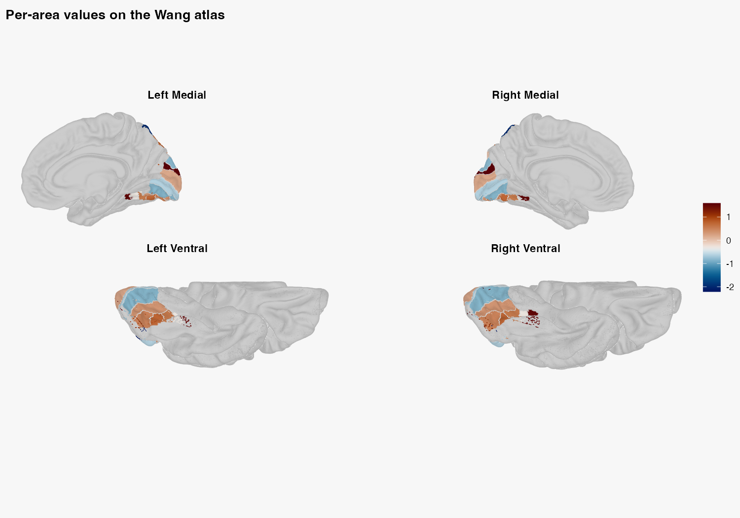
Supply one value for every region ID. To pair homologous labels across hemispheres, map by label explicitly rather than assuming the two halves share an accidental row order:

set.seed(1)
area_values <- stats::setNames(
  stats::rnorm(length(unique(wang$labels))),
  unique(wang$labels)
)
values <- unname(area_values[wang$labels])

stopifnot(
  length(values) == length(wang$ids),
  identical(
    values[wang$hemi == "left"],
    values[wang$hemi == "right"]
  )
)

plot_brain(
  wang,
  vals = values,
  views = c("medial", "ventral"),
  interactive = FALSE,
  style = "ggseg_like",
  background = TRUE,
  palette = "vik",
  colorbar = "right",
  colorbar_title = "Response (a.u.)",
  title = "Per-area values on the Wang atlas"
)

Synthetic area-level values mapped symmetrically onto medial and ventral views of the left and right Wang visual atlas, with a blue-to-orange response colorbar.

get_roi(wang, label = "hV4") returns one ROISurface per hemisphere. Use hemi = "left" or hemi = "right" when the analysis is unilateral.

How do you inspect the volume product safely?

A manifest is side-effect-free. It states the source, requested files, and whether those files are already cached:

library(neuroatlas)

manifest <- get_wang_prob_atlas(
  image = "maxprob",
  hemi = "both",
  path_only = TRUE
)

manifest$files[c("hemi", "member", "exists")]
#> # A tibble: 2 × 3
#>   hemi  member                             exists
#>   <chr> <chr>                              <lgl> 
#> 1 lh    subj_vol_all/maxprob_vol_lh.nii.gz FALSE 
#> 2 rh    subj_vol_all/maxprob_vol_rh.nii.gz FALSE

Set path_only = FALSE to download and read the volumes. The left and right label maps must share a grid and must not overlap before they are combined:

wp <- get_wang_prob_atlas(
  image = "maxprob",
  hemi = "both",
  path_only = FALSE
)

left <- as.array(wp$volumes$lh)
right <- as.array(wp$volumes$rh)

stopifnot(
  identical(dim(left), dim(right)),
  identical(
    neuroim2::space(wp$volumes$lh),
    neuroim2::space(wp$volumes$rh)
  ),
  !any(left > 0 & right > 0),
  all(unique(left[left > 0]) %in% wp$labels$id),
  all(unique(right[right > 0]) %in% wp$labels$id)
)

right[right > 0] <- right[right > 0] + 25L
labels <- neuroim2::NeuroVol(
  left + right,
  neuroim2::space(wp$volumes$lh)
)

Render the label map categorically on its native grid unless you have a validated anatomical reference in that same space. The zero background is omitted, and only areas present in the selected slices receive colours:

label_array <- as.array(labels)
occupied <- which(label_array > 0, arr.ind = TRUE)
slice_ids <- unique(as.integer(stats::quantile(
  occupied[, 3],
  probs = seq(0.08, 0.92, length.out = 6),
  type = 1
)))

x_limits <- pmax(
  1L,
  pmin(dim(label_array)[1], range(occupied[, 1]) + c(-7L, 7L))
)
y_limits <- pmax(
  1L,
  pmin(dim(label_array)[2], range(occupied[, 2]) + c(-7L, 7L))
)

slice_data <- do.call(rbind, lapply(slice_ids, function(z) {
  index <- which(label_array[, , z] > 0, arr.ind = TRUE)
  data.frame(
    x = index[, 1],
    y = index[, 2],
    region_id = label_array[cbind(index[, 1], index[, 2], z)],
    slice = factor(z, levels = slice_ids)
  )
}))

region_names <- c(
  stats::setNames(paste0(wp$labels$label, " (L)"), wp$labels$id),
  stats::setNames(paste0(wp$labels$label, " (R)"), wp$labels$id + 25L)
)
present_ids <- sort(unique(slice_data$region_id))
region_palette <- stats::setNames(
  grDevices::hcl.colors(length(present_ids), "Dynamic"),
  present_ids
)

wang_figure <- ggplot2::ggplot(
  slice_data,
  ggplot2::aes(x, y, fill = factor(region_id))
) +
  ggplot2::geom_tile(width = 1, height = 1) +
  ggplot2::facet_wrap(~slice, ncol = 3, labeller = ggplot2::label_both) +
  ggplot2::coord_fixed(xlim = x_limits, ylim = y_limits, expand = FALSE) +
  ggplot2::scale_fill_manual(
    values = region_palette,
    labels = region_names[as.character(present_ids)],
    name = NULL,
    drop = FALSE
  ) +
  ggplot2::labs(
    title = "Wang 2015 maximum-probability labels",
    subtitle = "Categorical areas on the native ProbAtlas_v4 voxel grid",
    caption = paste(
      "L and R identify hemisphere; numeric label order is not quantitative."
    )
  ) +
  ggplot2::theme_void(base_size = 11) +
  ggplot2::theme(
    legend.position = "bottom",
    legend.text = ggplot2::element_text(size = 6.5),
    legend.key.size = grid::unit(0.28, "lines"),
    legend.key.width = grid::unit(0.75, "lines"),
    legend.box = "horizontal",
    plot.title = ggplot2::element_text(
      face = "bold", hjust = 0.5, size = 16
    ),
    plot.subtitle = ggplot2::element_text(hjust = 0.5, colour = "grey30"),
    plot.caption = ggplot2::element_text(hjust = 0.5, colour = "grey35"),
    strip.text = ggplot2::element_text(face = "bold", size = 10),
    panel.background = ggplot2::element_rect(
      fill = "white", colour = "grey85"
    ),
    plot.background = ggplot2::element_rect(fill = "white", colour = NA)
  ) +
  ggplot2::guides(
    fill = ggplot2::guide_legend(nrow = 3, byrow = TRUE)
  )

wang_figure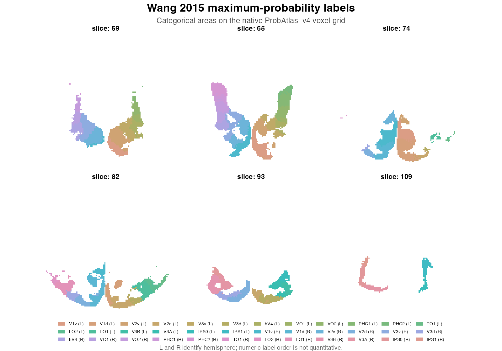

Six tightly cropped axial slices through the Wang maximum-probability maps on their native grid. Visual areas present in each slice have categorical colours and left or right hemisphere labels; zero background is white.

This figure deliberately has no unrelated T1 background. Nearest-neighbour resampling preserves integer labels on a new grid; it does not prove that an FSL-MNI product and a different MNI template are anatomically registered.

What about the other visual-cortex atlases?

get_visfatlas() loads the 33-region Rosenke et al. functional visual atlas on its distributed 1 mm single-subject MNI grid. Its provenance records alignment to MNI colin27. get_visual_atlas() derives V1-V5 regions from Julich-Brain. Both return ordinary volume atlas objects and can be rendered directly:

visf <- get_visfatlas()
plot(visf, nslices = 8, title = "visfAtlas on its distributed voxel grid")

julich_visual <- get_visual_atlas()
plot(julich_visual, nslices = 8, title = "Julich-derived V1-V5")

Do not resample visfAtlas onto MNI152NLin2009cAsym and call the result aligned: regridding is not a validated colin27-to-MNI2009 nonlinear transform. Inspect atlas_ref() and the transform plan before any cross-template overlay.

A representation checklist

Before analysis, record:

atlas product and citation;
surface or volume representation;
declared template and coordinate space;
region-ID convention, including hemisphere offsets;
any transform applied, with interpolation method and provenance.

That record is what makes the surface and volume versions scientifically traceable rather than merely visually similar.

References

Wang, L., Mruczek, R. E. B., Arcaro, M. J., & Kastner, S. (2015). Probabilistic Maps of Visual Topography in Human Cortex. Cerebral Cortex, 25(10), 3911-3931.

Rosenke, M., van Hoof, R., van den Hurk, J., Grill-Spector, K., & Goebel, R. (2021). A Probabilistic Functional Atlas of Human Occipito-Temporal Visual Cortex. Cerebral Cortex, 31(1), 603-619.